Continuum Mechanics
Introduction
Review of Equations of Mechanics: kinetics, kinematics, thermodynamic principles, constitutive equations, boundary-value problems of mechanics, equations for bar, beams, torsion and plane elasticity.
Bars and Beams: theory and applications.
Isotropic Plane Elasticity: Muskhelishvili's complex potentials, application to fracture mechanics.
Anisotropic Plane Elasticity: LES formalism, application to fracture mechanics.
Energy and Variational Principles: virtual work and energy principles, Hamilton's principle, energy theorems of structural mechanics, Castigliano's theorems, Betti's and Maxwell's theorems.
Variational Methods: Ritz's method, Galerkin's method, FEM.
References
Mathematical preliminaries
\(\boldsymbol{v}=v_i=(v_1,v_2,v_3)\) - vector, \(v_i\) for \(i=1,2,3\) are also the components of the vector \(\boldsymbol{v}\).
Lecture 1
Kinetics - Stress at Point
Forces acting on a body can be classified as internal and external. The internal forces resist the tendency of one part of the body to be separated from another part. The external bodies are those transmitted by the body. The external forces can be classified as body forces and surface forces. Body forces act on the distribution of mass inside the body. Examples of body forces are provided by the gravitational and magnetic forces. Body forces are usually measured per unit mass or unit volume of the body. Surface forces are contact forces acting on the boundary surface body. Example of surface forces are provided by applied forces on the surface of the body. Surface forces are reckoned per unit area.
Consider a body occupying the volume \(\Omega\) and bounded by surface \(S\). The surface force per unit area acting on an elemental area \(dS\) is called the traction or stress vector acting on the element. Consider the surface force \(\boldsymbol{f}\) acting on a small portion \(\Delta S\) of the surface surface area \(S\) of the body. The stress vector at a point \(P\) on \(\Delta S\) is defined by
Since the magnitude and direction depend on the orientation of the plane that created the surface, we denote it by \(\boldsymbol{t}^{(\boldsymbol{n})}\), where \(\boldsymbol{n}\) denotes the normal to the plane. The component of \(\boldsymbol{t}\) that is in the direction of \(\boldsymbol{n}\) is called the normal stress. The component of \(\boldsymbol{t}\) that is normal to \(\boldsymbol{n}\) is called shear stress. Let \(\boldsymbol{t}^{(i)}\) denote the stress vector at point \(P\) on a plane perpendicular to \(x_{i}\)-axis, then
where \(\sigma_{ij}\) denotes the component of stress vector \(\boldsymbol{t}^{(i)}\) along the \(x_{j}\)-direction. The state of stress at a point is characterized, in general, by nine components of stress \(\sigma_{ij}\).
The relationship between the stress vector \(\boldsymbol{t}^{(n)}\) acting on a plane given by normal \(\boldsymbol{n}\) and the stress vectors on three planes perpendicular to the coordinate axes \(x_{j}\) is called the Cauchy stress formula
which can be written in matrix form as
where \([\cdot]^{T}\) denotes the transpose of the matrix. The normal and shearing components of the stress vector \(\boldsymbol{t}^{(\boldsymbol{n})}\) are given by
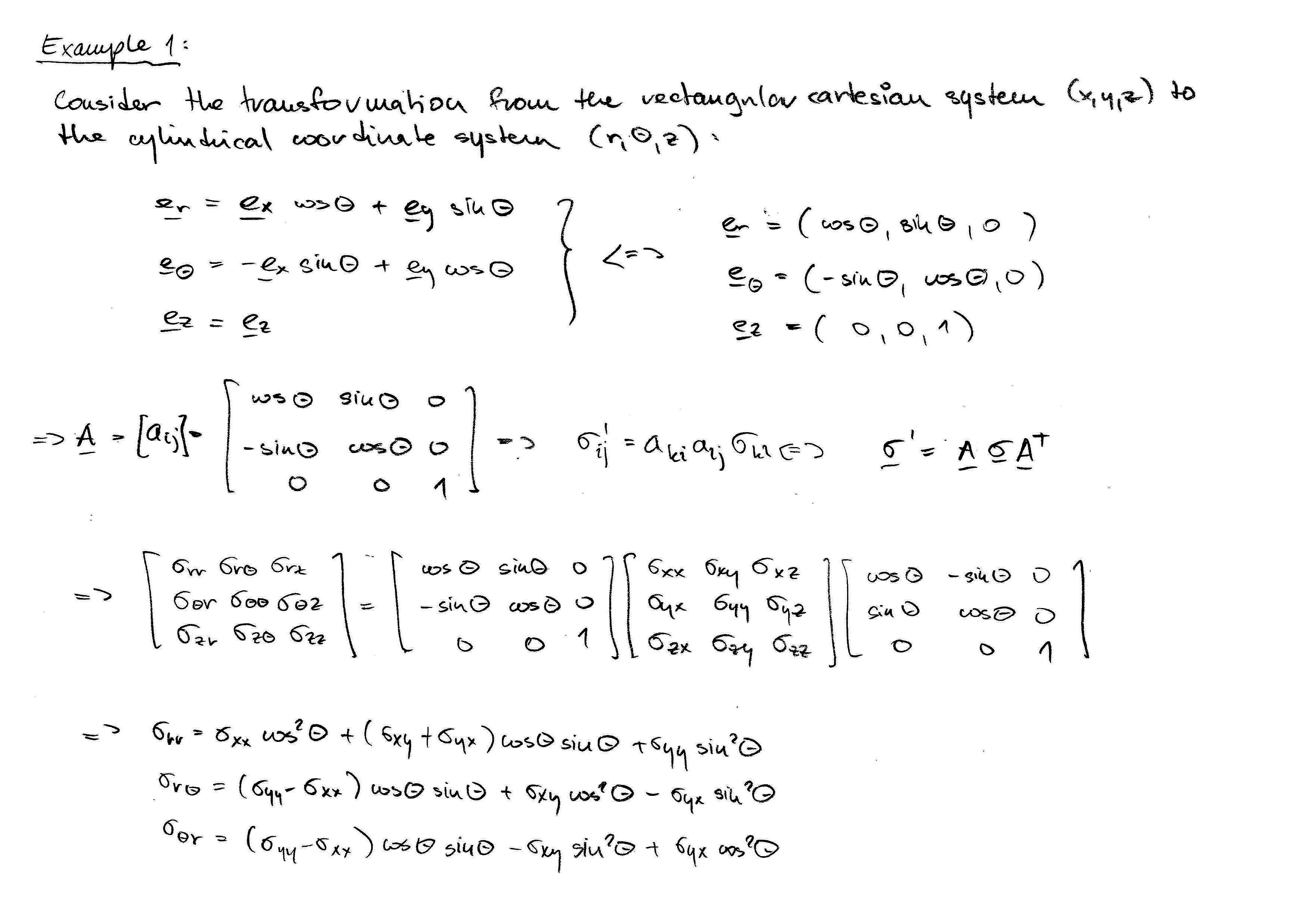
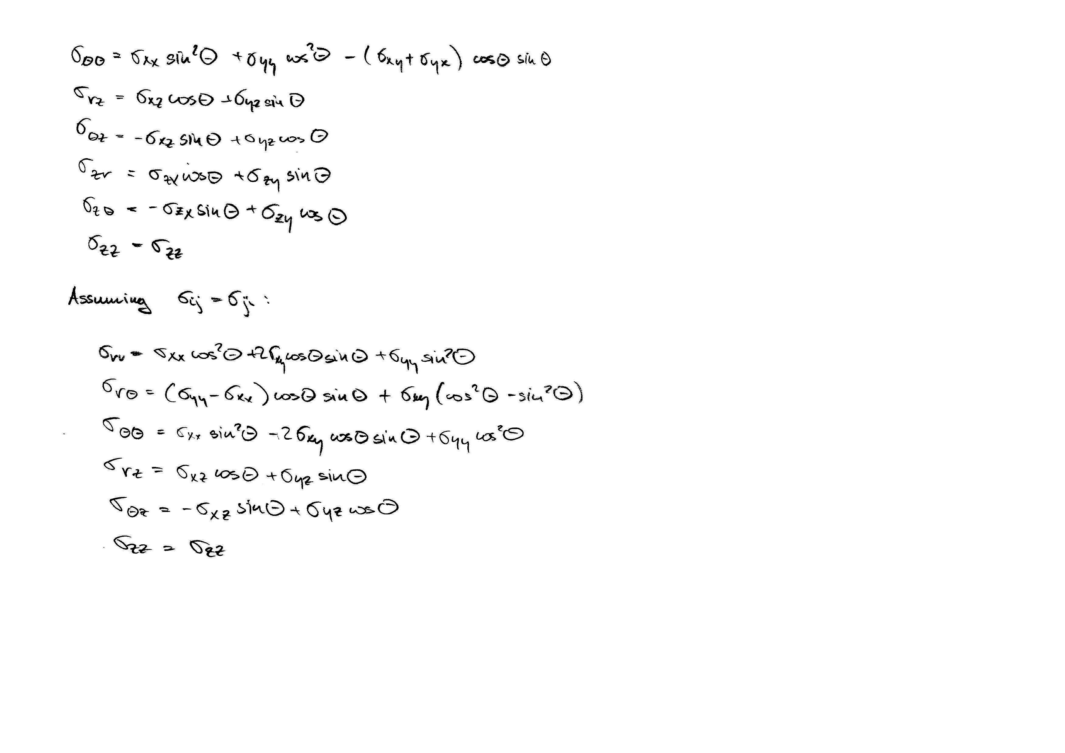
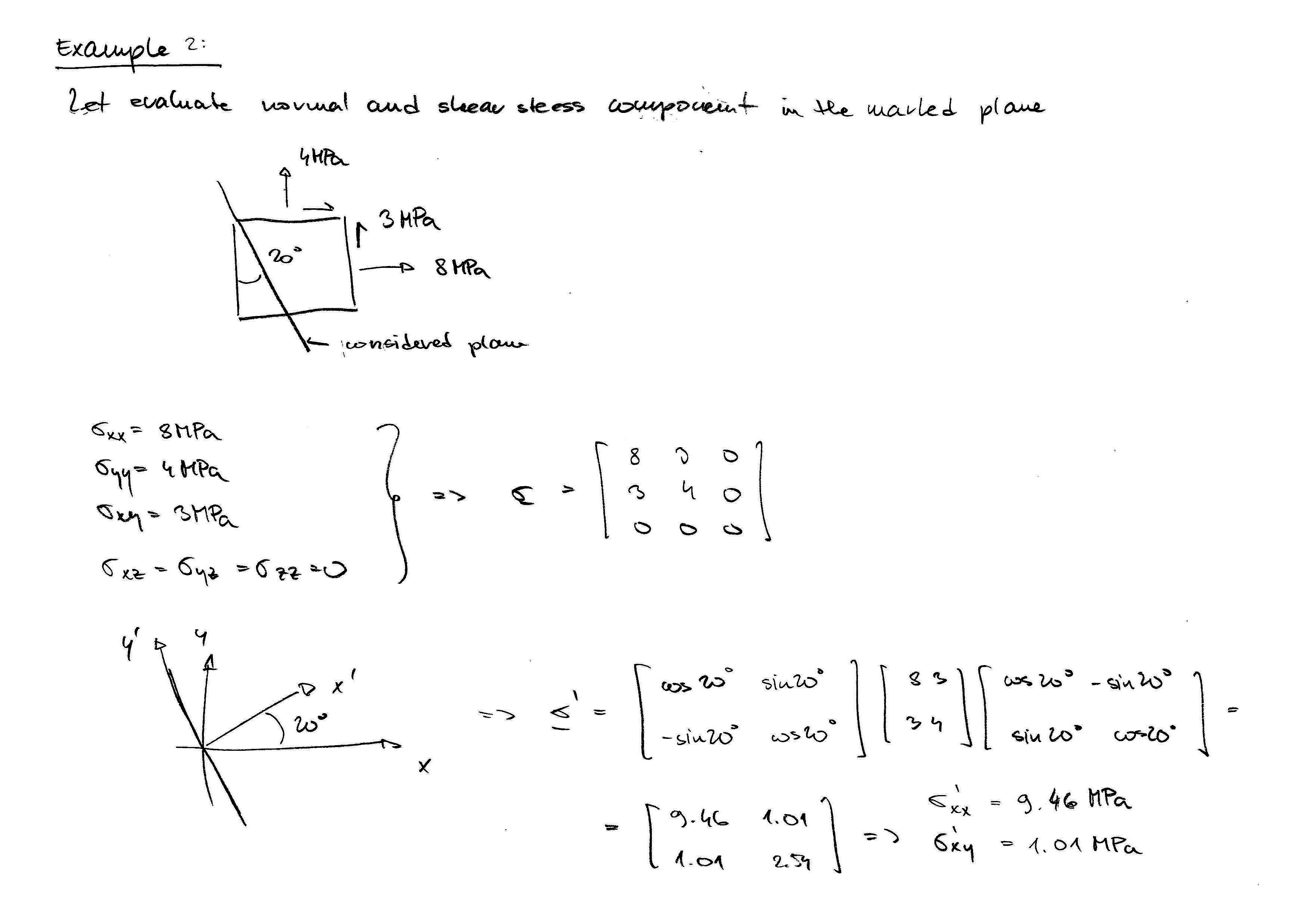
When the components of stress are known in one coordinate system, it is of interest to determine the components of stress in another coordinate system. The relationship between the components of stress tensor in one coordinate system and the components in another coordinate system is known as the transormation of stress. Such transformations are useful in determining the maximum values of normal and shear stresses and the planes on which they act. Consider two sets of orthogonal coordinate systems \((x_1,x_2,x_3)\) and \((x_1^\prime,x_2^\prime,x_3^\prime)\). Let \((\boldsymbol{e}_1,\boldsymbol{e}_2,\boldsymbol{e}_3)\) and \((\boldsymbol{e}_1^\prime,\boldsymbol{e}_2^\prime,\boldsymbol{e}_3^\prime)\) denote the sets of basis vectors in the two coordinate systems. Suppose that the two coordinate systems are related by the transformation equation
where \(a_{ij}\) denote the directions cosines
We note that the stress dyadic
at a point is invariant, that is does not depend on the coordinate system. However, the components do depend on the coordinate system. We have
and
From which follows
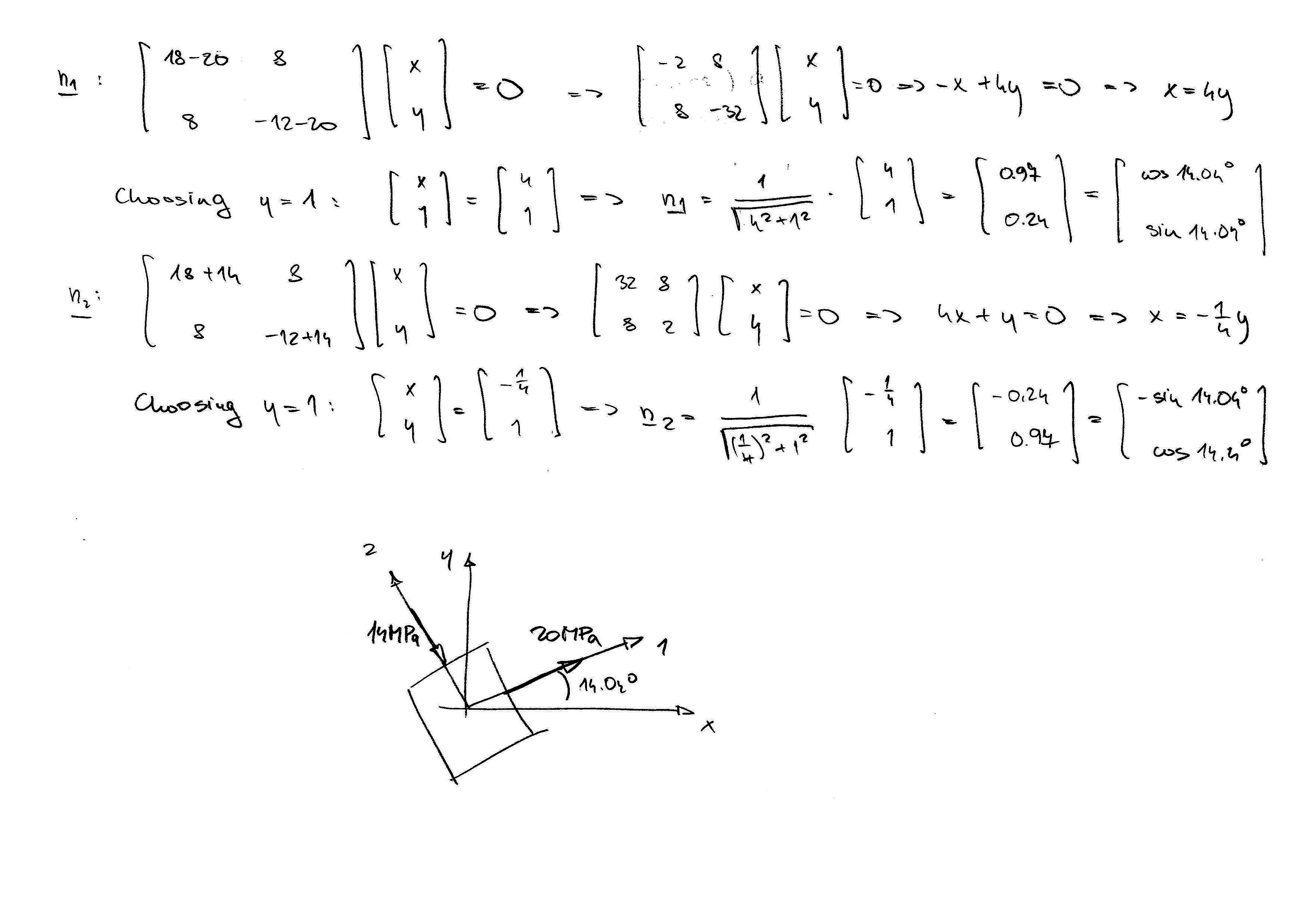
The question of finding the maximum and minimum normal stresses, called principal stresses, at a point is the considerable interest. The maximum normal stress at a point acts in a plane on which the shear stress is zero and consequently
where \(\lambda\) denotes the magnitude of the normal stress and \(\boldsymbol{n}\) denotes the unit normal to the plane on which the maximum stress is acting. This formula can also be written as
Equating these two equations, we obtain
or in component form
where \(\delta_{ij}\) is a Kronecker delta
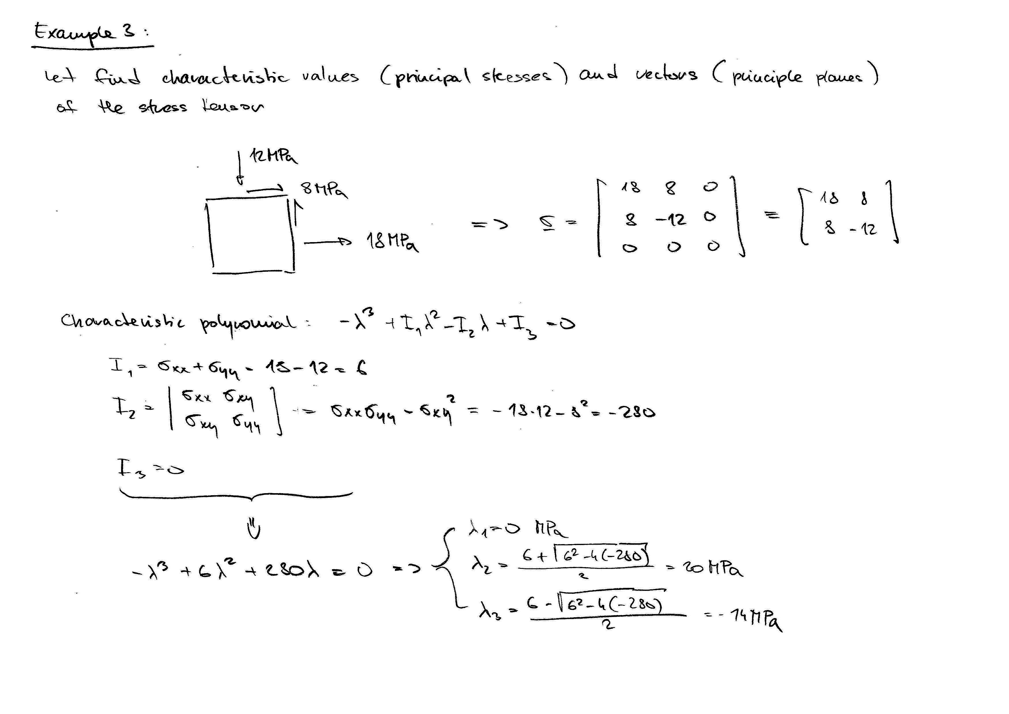
Equation (16) has a nontrivial solution (\(n_i\neq 0,i=1,2,3\)) only if the determinant of the coefficient matrix is zero
The determinant leads to the polynomial called characteristic and the three values of \(\lambda\) are called characteristic values or eigenvalues and associated (unit) normal vectors \(\boldsymbol{n}\) are called characteristic vectors or eigenvectors. The characteristic polynomial (18) is of the form
where \(I_1\), \(I_2\) and \(I_3\) are stress invariants defined as
For symmetric tress dyadic \(\boldsymbol{\sigma}\), i.e. \(\sigma_{ij}=\sigma_{ji}\), the eigenvalues are real.
Equations of Equilibrium
The equation of motion for solids can be derived from the principle of of conservation of linear momentum, which says that the time rate of change of the total momentum of a given body equals the vector sum of all the external forces acting on the body and provides the Newton's third law of action and reaction governs the internal forces. The momentum of the elemental volume \(d\Omega\) is \((\mathrm{mass}\times\mathrm{velocity})=(\rho d\Omega)\partial\boldsymbol{u}/\partial t\). The total momentum is given by
The time rate of the momentum is
where \(d/dt\) denotes the total (material) time derivative. The first integral on the right-hand side is equal to zero because of the principle of conservation of mass of a given material
The momentum principle can now be expressed as
where the external forces \(\boldsymbol{f}\) and \(\boldsymbol{t}\) are the body force and surface traction, respectively. Using equation (14), the stress vector \(\boldsymbol{t}\) can be expressed in terms of the stress tensor (dyadic) \(\boldsymbol{\sigma}\) and unit normal \(\boldsymbol{n}\). We obtain
Using the divergence theorem, the surface integral can be converted to a volume integral
The equation should hold for arbitrary region \(\Omega\). This implies that the integrand of the left-hand side of (26) should be identically equal to zero. This gives the vector from of the equation of motion
In a rectangular cartesian coordinate system, this equation takes the form
The equations of equilibrium are obtained by setting the right-hand side of (27) equal to zero
When a body is not subjected to distributed couples (i.e., volume-dependent couples are not present), one can establish the symmetry of the stress tensor using the Newton's second law for moments or using the principle of moment of momentum. Both methods give the result
where \(\epsilon_{ijk}\) is the permutation symbol
Or rewritten to the components
Thus, there are only six stress components that are independent. Because (27) contains three equations relating six stress components, the equations of equilibrium are not sufficient for the determination of the stress components. Additional equations are required, the strain-displacement equations and constitutive equations.
Lecture 2
Kinematics - Strain at Point
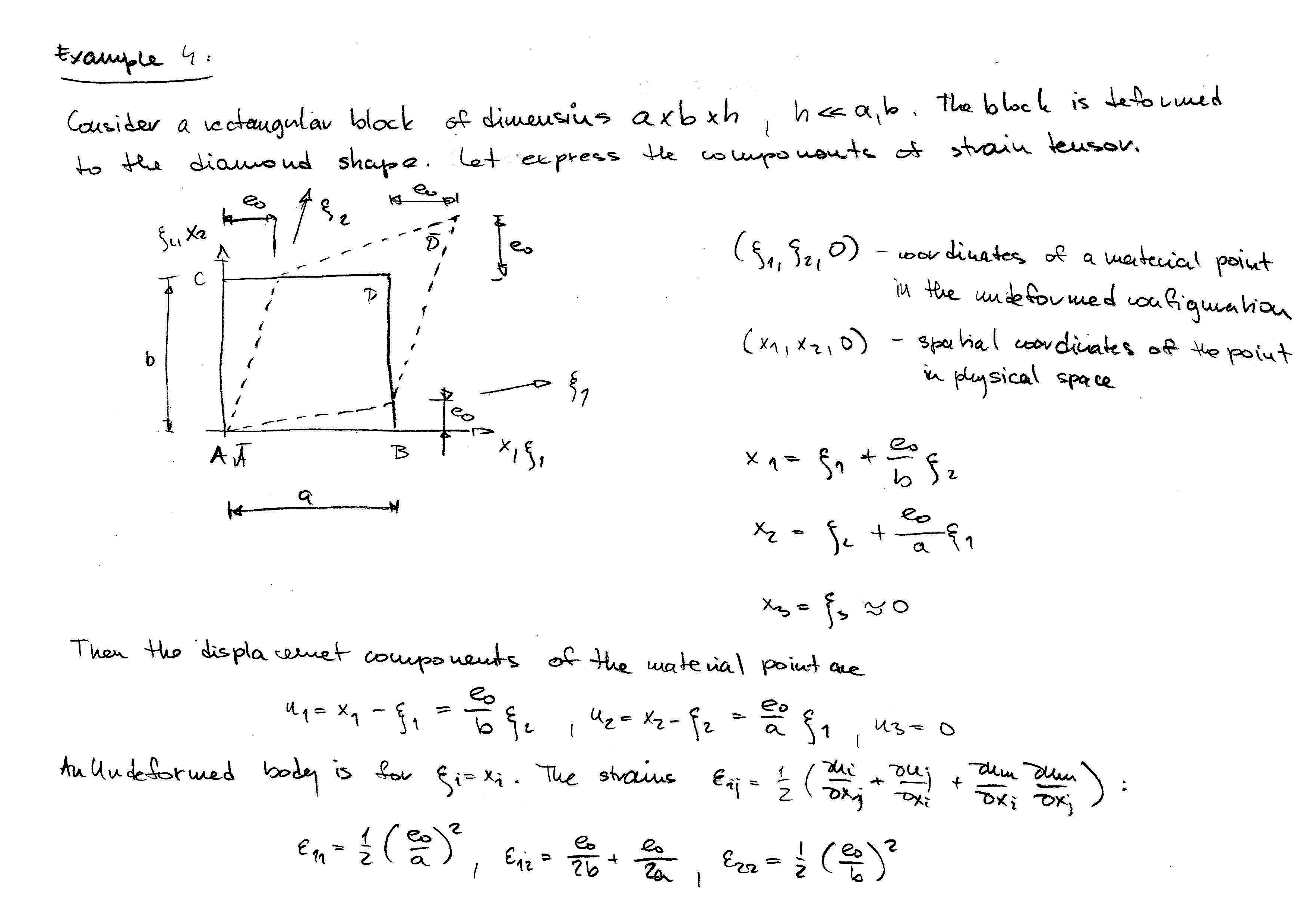
To describe the motion of a deformable body, we establish a fixed reference frame in three dimensional space and denote the Cartesian coordinates of a point be \(\boldsymbol{x}=(x_1,x_2,x_3)\). A measure of the deformation in a body is provided by the change in the distance between points in the body. Consider two neighboring points \(P=(x_1,x_2,x_3)\) and \(Q=(x_1+dx_1,x_2+dx_2,x_3+dx_3)\) in the reference configuration. Under the action of externally applied forces, the body deforms and the points \(P\) and \(Q\) move to new places \(\overline{P}=(\xi_1,\xi_2,\xi_3)\) and \(\overline{Q}=(\xi_1+d\xi_1,\xi_2+d\xi_2,\xi_3+d\xi_3)\), respectively. Since points \(P\) and \(Q\) are arbitrary, the discussion applies to any point in the body. The motion of a particle occupying position \(\boldsymbol{x}\) in the undeformed body to point \(\boldsymbol{\xi}\) in the deformed body can be expressed by the transformation
where \(t\) denotes time. By assumption a continuous medium cannot have gaps or overlaps. Therefore, a one-to-one correspondence exists between points in the undeformed body and points in the deformed body. Consequently, a unique inverse to (33) holds
If the distances between points \(P\) and \(Q\) is \(ds\) and the distance between points \(\overline{P}\) and \(\overline{Q}\) is \(d\overline{s}\), then the measure of deformation of the body is
where \(\varepsilon_{ij}\) are the components of the Green strain tensor at point \(P\)
The symbol \(\delta_{ij}\) is a Kronecker delta (17). The displacements can be written as
The substitution of the last expression to (36) gives the expression of strains in terms of the displacements at point \(P\)
We will assume in the following that the displacement components are small compared to unity, i.e.
then strain components \(\varepsilon_{ij}\) become the infinitesimal strain componets
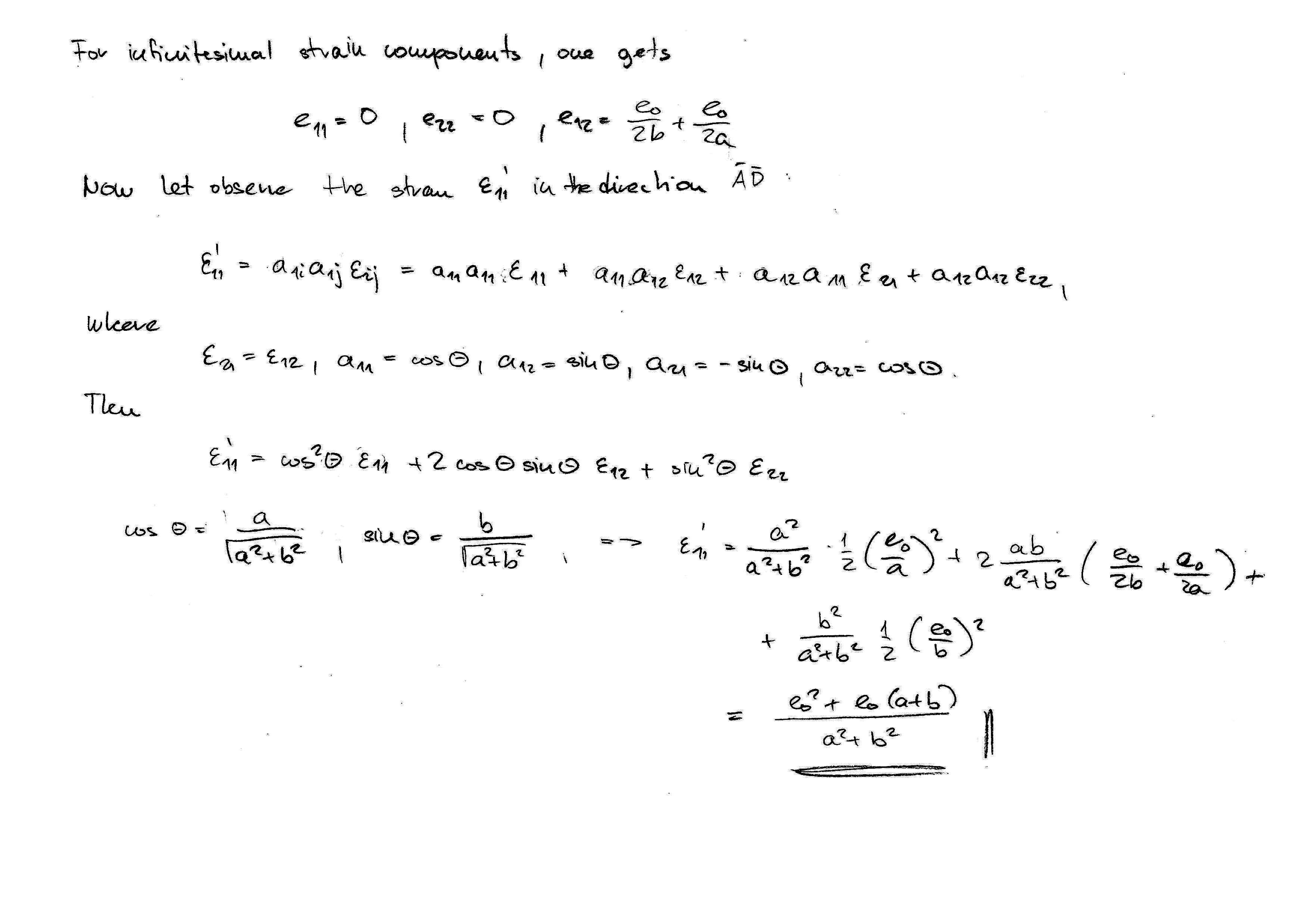
Similarly to the stresses at a point, it is a matter of interest to know the components of strain at a point in one coordinate system, e.g. \((x_1^\prime,x_2^\prime,x_3^\prime)\), if they are known in the another coordinate system \((x_1,x_2,x_3)\) at the same point. It is not difficult to proof, that the tensor character of strain is associated with the transformation relation
where
Compatibility Conditions
When the strain components are given, the determination of the displacements is not always possible, because there are six strain components related to three displacement components. Stated in other words, there are six differential equations involving three unknowns. Thus, the six equations should be compatible with each other in the sense that any three equations should give the same displacement field. Assuming the infinitesimal strain components, the only way, how to connect six partial differential equation (40) and eliminate the components of displacements appearing in them, is to derive them two times. Then it can be observed
Equation (43) forms the necessary and sufficient conditions for the existence of a single-valued displacement field (when the strains are given). It is 81 equations, but only six of them are non trivial and different and linearly independent from each other
Lecture 3
First Law of Thermodynamics
The first law of thermodynamics is commonly known as the principle of balance of energy and it can be regarded as a statement of the interconvertibility of heat and work. The law does not place any restriction on the direction of the process. The first law of thermodynamics states that the time-rate of change of the total energy (i.e. sum of the kinetic energy and the internal energy) is equal to the sum of the rate of work done by the external forces and the change of heat content per unit time
where \(K\) denotes the kinetic energy, \(U\) is the internal energy, \(W\) is the power input and \(H\) is the heat input to the system. The kinetic energy of the system is given by
If \(\hat{U}_0\) is the energy per unit mass (or specific internal energy), the total internal energy of the system is given by
The kinetic energy \(K\) of a system is the energy associated with the macroscopically observable velocity of the continuum. The kinetic energy associated with the microscopic motions of molecules of the continuum is a part of the internal energy. The elastic strain energy and other forms of energy are also parts of internal energy.
The power input in the nonpolar case, consists of the rate at which the external surface tractions \(\boldsymbol{t}\) per unit area and body force \(\boldsymbol{f}\) per unit volume are doing work on the mass system instantaneously occupying the volume \(\Omega\) bounded by \(S\)
where \(:\) denotes the double-dot product of tensors. The expression (49) can be rewritten to the form
The rate of heat input consists of conduction through the surface \(S\) and internal heat generation in the body
where \(\boldsymbol{q}\) is the heat flux vector normal to the surface and \(Q\) is the internal heat source per mass. Substituting (47), (48), (50) and (51) into (46), we obtain
or
for arbitrary volume \(\Omega\). Let us denote
then the conservation of energy implied by the first law of thermodynamics is given as
Second Law of Thermodynamics
From our experience we know, that mechanical energy that is converted into heat cannot be converted back into mechanical energy. Although the first law of thermodynamics does not restrict the reversal process, namely the conversion of heat to internal energy and internal energy to motion, such a reversal cannot occur because the frictional dissipation is an irreversible process. In addition to the first, the second law adopts these features. The second law of thermodynamics for a reversible process states, that there exits a function \(\eta=\eta(Q,\boldsymbol{q},T)\) called the specific entropy, such that
is a perfect differential. Equation (56) is called the entropy equation of state. Combining (55) and (56) we arrive at the equation
For irreversible processes, the second law of thermodynamics states that (56) is not total differential, but
which is known as the Clausius-Duhem inequality.
Downloads 3:
Lecture 3 to download
hereas the pdf presentation.
Lecture 4
Generalized Hook's Law
A material body is said to be ideally elastic when the body recovers (under isothermal conditions) its original form completely upon removal of the forces causing deformation and there is a one-to-one relationship between the state of stress and state of strain. The generalized Hook's law relates the nine components of stress to the nine components of strain by the linear relation
where \(e_{kl}\) are the infinitesimal strain components, \(\sigma_{ij}\) are Cauchy stress components and \(c_{ijkl}\) are the material parameters. A material is said to be homogeneous if the parameters \(c_{ijkl}\) do not vary from point to point in the body. The nine equations in (59) contain 81 parameters. However, owing to the symmetry of both \(\sigma_{ij}\) and \(e_{kl}\), it follows that
and there are only 36 constants. Equation (59) can also be expressed in the matrix form
or
where
Hence, the rules apply to indexes in (61) are
Note that \(\sigma_i\) and \(e_j\) do not constitute the components of tensor. Therefore one cannot transform the components \(\sigma_i\) and \(e_i\) like vectors, but these must be rewritten to the tensor components \(\sigma_{ij}\) or \(e_{kl}\), transformed and consequently written to the vector form. The same rule is valid for matrix components \(c_{ij}\).
Strain Energy Density Function
In ideal elasticity, when \(\eta\) is differentiable and \(d\eta=0\), it is assumed that all of the input work is converted into internal energy in the form of recoverable stored elastic energy. If we denote the strain energy per unit volume by \(U_0=U_0(e_{ij})\), then from (57) follows
When temperature effects are involved, the strain energy density is a function of strains and temperature \(U_0=U_0(e_{ij},T)\) and it must be introduced the free-energy function \(\Psi\) combining the strain energy density \(U_0\) and entropy \(\eta\) to be treated as the potential
Since \(\Psi\) is a function of the strains \(e_{ij}\) and temperature \(T\), we have
Substituting (57) into (68) yields
Because the differentials \(de_{ij}\) and \(dT\) are independent to each other, the previous equation leads to the relations
From (66) and (70) also follows important result, if the deformation process is isothermal and reversible, i.e. the temperature \(T\) is constant during the very slow quasi-static process in the thermodynamic equilibrium, then
The first relation from (71) can be used to reduce the number of independent elastic constants to 21. The substitution of the generalized Hook's law (59) into the first equality in (71) gives
The partial differentiation of (72) with respect to \(e_{kl}\) gives
The interchanging the indices \(kl\) with \(ij\) we obtain
Since the order of partial differentiation is unimportant, it follows that
The importance of this result is that it was obtained from the thermodynamics considerations without any symmetry requirements to the stress or strains tensors \(\sigma_{ij}\) or \(e_{ij}\), respectively. Consequently the array \(c_{ij}\) in (62) is symmetric and the number of independent constants is reduced from 36 to 21.
It is also useful to introduce the thermodynamic potential \(\Psi^*\) as follows
for which yields
Analogically to the previous derivations, the strain components \(e_{ij}\) can be evaluate for the isothermal deformations process as
Elastic Symmetry
The elastic moduli \(c_{ij}\) relating the cartesian components of stress and strain depend on the orientation of the coordinate system. When \(c_{ij}\) do not depend on the orientation, the material is isotropic for which the stress-strain relationship is of the form
where \(\mu\) and \(\lambda\) are called Lamé constants. The Lamé constants are related to the shear modulus \(G\), Young's modulus \(E\) and Poisson's ratio \(\nu\) by
The coefficients \(c_{ij}\) for isotropic materials have the following meaning
and all other \(c_{ij}\)'s are zero.
Whenever three mutually orthogonal planes of elastic symmetry for a material exist, the material is said to be orthotropic. In this case, the coefficients \(c_{ij}\) are as follows
where \(E_1\), \(E_2\), \(E_3\) are Young's moduli in 1, 2 and 3 directions, \(\nu_{ij}=-e_{jj}/e_{ii}\) are Poisson's ratios of transverse strain in the \(j\)-direction to the axial strain in the \(i\)-direction, when stressed in the \(i\)-direction and \(G_{23}\), \(G_{13}\), \(G_{12}\) are shear moduli in the 2-3, 1-3 and 1-2 planes. More convenient it is used the components of the compliance matrix \(\boldsymbol{S}\), which is inverse to the stiffness matrix (61) and obeys the relation
or in tensor form
where
It is of interest in the study of laminated plates of orthotropic layers to have an explicit form of the transformation equations relating the elastic moduli in one coordinate system to those in another coordinate system. The parameters \(c_{ijkl}\) are components of a fourth-order tensor and similarly to the transformation equations (12) and (41) for tensors, the tensor \(c^\prime_{ijkl}\) is transformed as
where \(a_{im}\) denotes the direction cosines associated with the \(x^\prime_i\)-axis and the \(x_m\)-axis
Deformations Due to Temperature Change and Thermoelastic Constitutive Equations
A change in the temperature of a body leads to its deformation due to the thermal expansion, even if there is no external load acting on it. When the thermal expansion are prevented by boundary conditions or other constrains, the body develops also the thermal stresses in addition to stresses caused by other loads. In this case, the temperature \(T\), measured above an arbitrary reference temperature \(T_0\), enters as a parameter in the linear terms of strains \(e_{ij}\) of the free energy
Following (70), the linear thermoelastic constitutive equations and entropy are given by
and
where \(\beta_{ij}\) are the Cartesian components of the tensor \(\boldsymbol{\beta}\) representing the material thermal expansion parameters. For an isotropic body equation (93) and (94) take the simple forms
where
and \(\alpha\) is the linear coefficient of thermal expansion. Setting the stresses on the left-hand side in the first expression of (95) equal to zero, then it is obtained
The isothermal deformation process of the body will be considered in the following elasticity problems and applied variational methods. It means, that the temperature of the deformed body during its quasi-static deformation process must be constant, i.e. \(T=T_0\). Then the first equation in (95) is reduced to the standard constitutive relation for isotropic material
As the consequence, the material parameters \(\lambda\) and \(\mu\) are known as isothermal. On the other hand, the relations (71) show that the stress tensor \(\sigma_{ij}\) in an isothermal process can be evaluated as the derivative of the deformation energy \(U_0\) with respect to the deformations, if the entropy \(\eta\) is constant. Constant entropy \(\eta\) is associated with an adiabatic process, i.e. a very fast thermodynamic process during which the body does not have time to exchange its temperature \(T\) with the surroundings across the boundary. The expression for the entropy in (95) is constant only if the temperature change \(T-T_0\) is nonzero and proportional to the first deformation invariant \(e_{kk}\), i.e.
This condition is equivalent to the equation (97) for the deformations during the isothermal process and zero stresses \(\sigma_{ij}\). The substitution of temperature \(T-T_0\) from (99) into the free energy \(\rho\Psi\) in (92), it is obtained the strain energy density \(U_0\), which can be written in the form
where \(c^{ad}_{ijkl}=c^{ad}_{ijkl}(T)\) are the adiabatic elastic parameters linearly depending on the temperature \(T\). Supposing the isotropic material and applying the second relation of (71), it is obtained
In practice, the dependence of \(c^{ad}_{ijkl}=c^{ad}_{ijkl}(T)\) on the temperature \(T\) is very weak and we can assume that the difference between \(c^{ad}_{ijkl}\) and \(c_{ijkl}\) can be neglected. This assumption allows us to handle the thermoelastic constitutive problem in an elegant mathematical way. We will therefore assume a quasi-static loading process, i.e. an isothermal process, that is always in thermodynamic equilibrium. However, the stress tensor components \(\sigma_{ij}\) are calculated from the strain energy density \(U_0\) under the condition of constant entropy \(\eta\), i.e. the adiabatic thermodynamic process, according to the equation (66). If we omit the unnecessary notation \(\eta=const\), we get
with additional deformation condition (97). It will be supposed that the strain energy density \(U_0\) is independent of the temperature \(T\), it is conservative, differentiable and reversible. Similarly, the so-called complementary strain energy \(U^*_0\) can be introduced to the evaluation of the strains \(e_{ij}\) in the isothermal process using the thermodynamic potential \(\Psi^*\) defined in (76) and its application in relation (78). The complementary strain energy \(U^*_0\) is defined as follows
and according to the previous assumptions and derivations, we will calculate the strains \(e_{ij}\) in the isothermal process as follows
Downloads 4:
Lecture 4 to download
hereas the pdf presentation.
Lecture 5
Boundary-Value Problems of Mechanics
We summarize the equations mentioned above
Equation of motion
Strain-displacement equations
Linear constitutive relations
Thus, there are 15 unknowns and 15 equations for a three-dimensional elastic body, which should be solved in conjunction with appropriate initial and boundary conditions
Variables |
Number |
|---|---|
\(\boldsymbol{u}\), \(u_i\) |
3 |
\(\boldsymbol{e}\), \(e_{ij}\) |
6 |
\(\boldsymbol{\sigma}\), \(\sigma_{ij}\) |
6 |
For a three-dimensional elastic body, the initial and boundary conditions are of the following form
Initial conditions (\(t=0\), \(\boldsymbol{x}\) or \(x_i\) inside the body)
Boundary conditions (\(t\ge0\), \(\boldsymbol{x}\) or \(x_i\) on the boundary)
Here, variables with a superscript or subscript zero denote the specified initial values and those with a caret over them denote the specified boundary values of the variables.
Solving the 15 equations (105)-(107) for the 15 unknowns in conjunction with the initial and boundary conditions in (108)-(110) is of primary interest in solid mechanics. We can classify the formulations into the following three categories (for isothermal case):
Displacement Formulation (Boundary-Value Problem of the First Kind). This formulation involves the determination of displacements and stresses in the interior of the body under a given body force distribution and specified displacement field over the entire boundary of the body.
Stress Formulation (Boundary-Value Problem of the second Kind). This problem entails the determination of displacements and stresses in the interior of the body under the action of a given body force distribution and specified surface forces on the entire boundary.
Mixed Formulation (Boundary-Value Problem of the Third Kind. This requires the determination of displacements and stresses in the interior of the body under the action of a given body force distribution and specified displacement field on a portion of the boundary and specified boundary forces on the remaining portion of the boundary of the body.
For boundary-value problem of the first kind, it is convenient to express all of the governing equations in terms of the displacement field \(u_i\). This is done by eliminating stresses \(\sigma_{ij}\) in the equations of motion (105) by substitution of the stress-strain equations (107) and then eliminating the strains \(e_{ij}\) by the strain-displacement equations (106). The initial and boundary conditions are given by (108) and (109), respectively. For an isotropic body with \(T=T_0\), the governing equations have form
or
These equations are called the Navier equations of motion.
For boundary-value problems of the second kind, we find that it is convenient to write the governing equations (105) in terms of stresses \(\sigma_{ij}\). It is the simplest boundary value problem in the case of an isothermal loading process, suitable for finding a solution in analytical form. The equations of motion (105) are reduced to the form
or
with prescribed natural boundary conditions (110). The extreme values of stress \(\sigma_{ij}\) are usually of interest in solved elasticity problems, but if the goal is also to know the deformations of the body \(e_{ij}\), it is necessary to solve additional differential equations given by the stress-strain equations (107) and the deformation-strain equations (106) to obtain the displacements \(u_i\). The displacements \(u_i\) can be found uniquely, except for the rigid-body motion.
For the boundary-value problem of the third kind, the governing equations are given by (for \(t>0\))
or
with boundary conditions (109) on one portion and (110) on the remainder of the boundary. Most problems of solid mechanics fall under the third (i.e. mixed) category.
Existence and Uniqueness of Solutions
The existence and uniqueness of the solution of the above mentioned differential equations follows from the Lax-Milgram theorem, which assumes continuity and positive-definiteness of the operator in the governing differential equation (115), which in the case of its linearity and linearity of stress-strain relations is satisfied. Suppose that \(u_i^1\) and \(u_i^2\) are two solutions of the same mixed boundary-value problem. We assume the following initial conditions and mixed boundary conditions
Then we have
or
where
Multiply (120) by \(\partial\overline{u}_i/\partial t\) and integrate first over the volume of the body and then with respect to time from initial time \(t_0\) to current time \(t\)
and consequently integrate per-partes
The surface integral in (123) vanishes, because
Moreover, it holds
Then we have
or
The second integral in (127) we set zero, because both strain and kinetic energy \(U_0\) and \(K\), respectively, are measured from initial values \(U_0(t_0)=\partial u(t_0)/\partial t=0\). Thus we have
Both
are quadratic functions of \(\overline{e}_{ij}\) and \(\partial\overline{u}_i/\partial t\) which implies that
These in turn require that
where \(k\) is an arbitrary constant. In other words, the displacements of the mixed boundary-value problem are unique within an arbitrary constant responsible for the rigid-body motion. However this constant must be equal zero, because both \(u_i^1\) and \(u_i^2\) are equal to \(\hat{u}_i\) on \(S_1\). From this follows the uniqueness of solutions. When \(u_i\) is not specified at any point of the boundary (like in the boundary-value problem of the second kind), the stresses \(\sigma_{ij}\) are unique but the displacements \(u_i\) are not and they differ by a rigid-body motion.
Equations of Bars, Beams, Torsion and Plane Elasticity
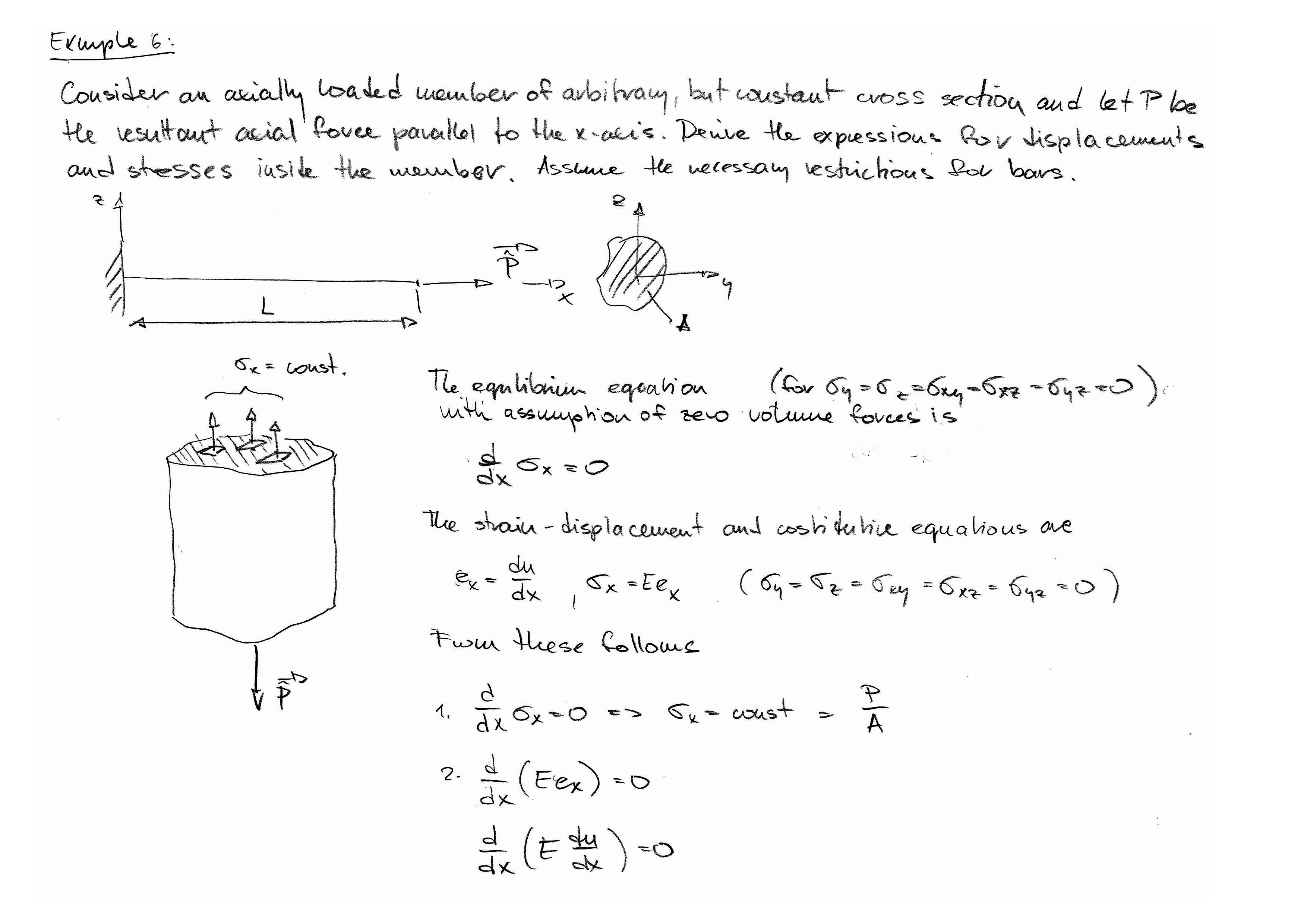
Axially Loaded Bars
The equations of axially loaded members are based on the assumption of an uniform stress distribution \(\sigma_x\) as a function of \(x\) alone and is independent of the position at any given section. The main restrictions of the theory of axially loaded members called bars are
The cross section of the member is arbitrary, but is either uniform or gradually varying in the axial direction. If sudden changes in the cross section are involved, the centroids of all cross sections can be joined by a straight line parallel to the axis of the member.
The material of the member is homogeneous or the modulus of elasticity \(E\) can be a function of the axial coordinate.
All applied loads and support points are geometrically positioned in line with the centroidal axis of the member.
The load magnitude in compression is less than the critical buckling load of the member.
The points of load application and support connections are at reasonable distances from the point of interest.
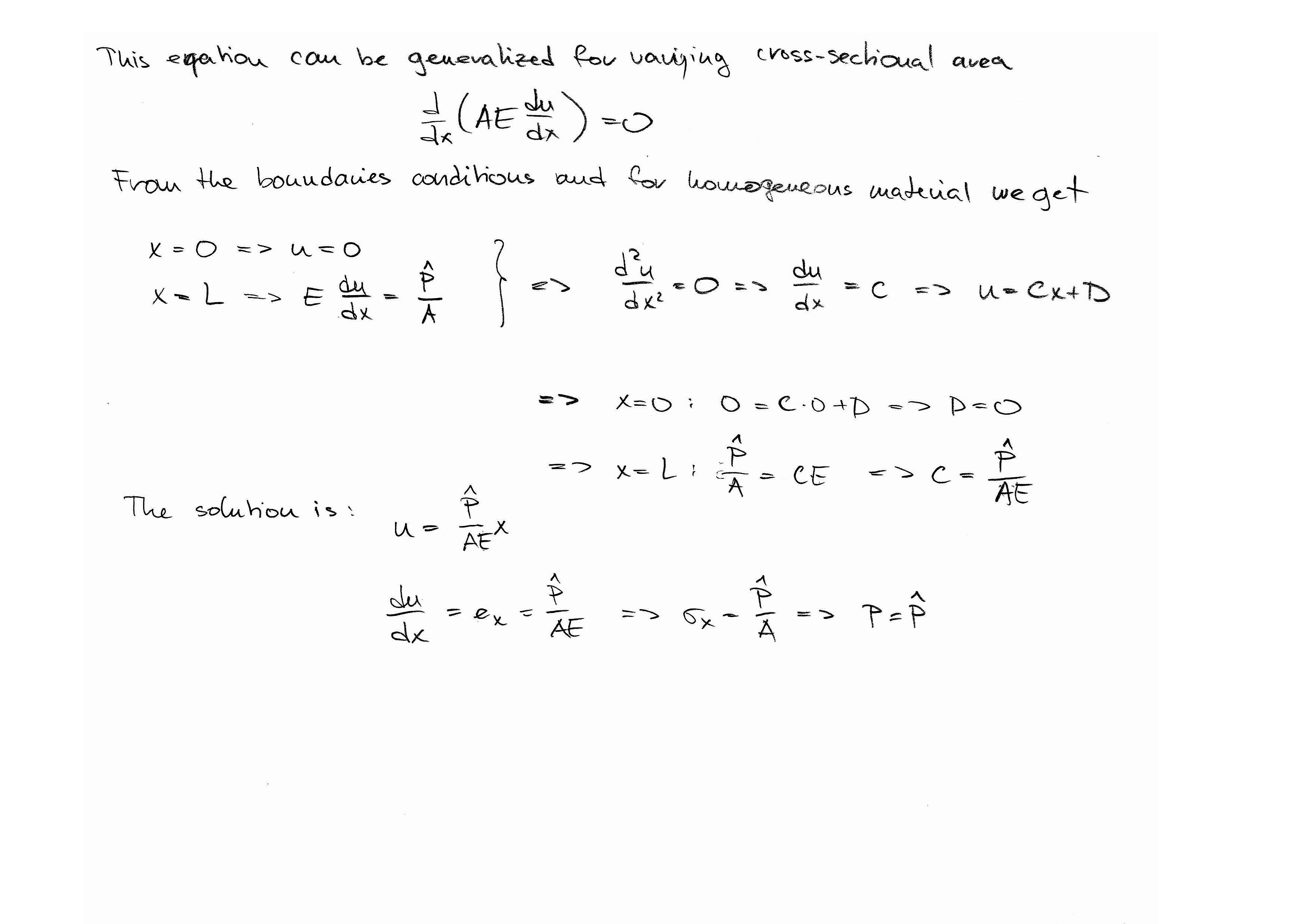
These restriction allows one to formulate the mixed boundary-value problem (115) to the form
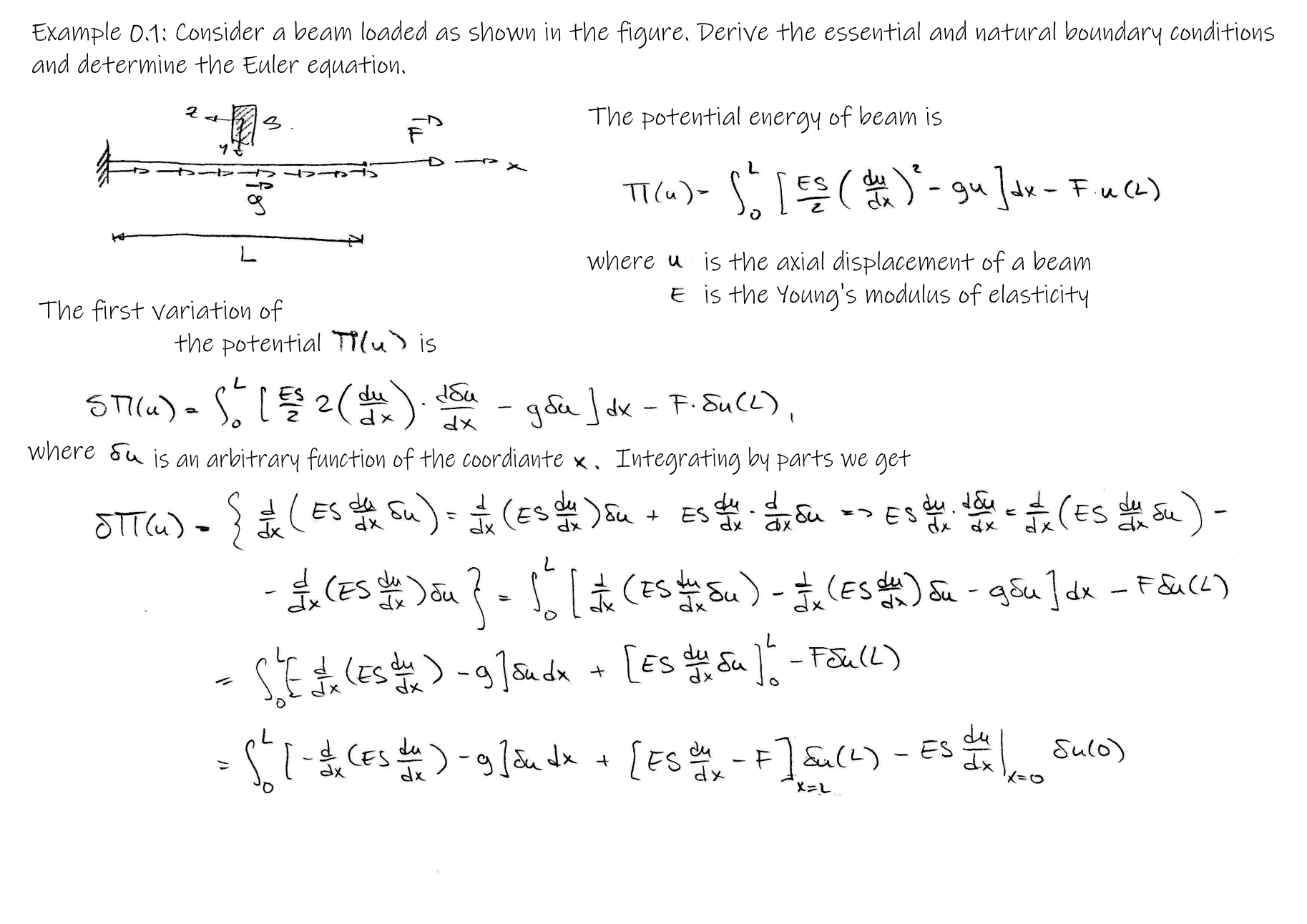
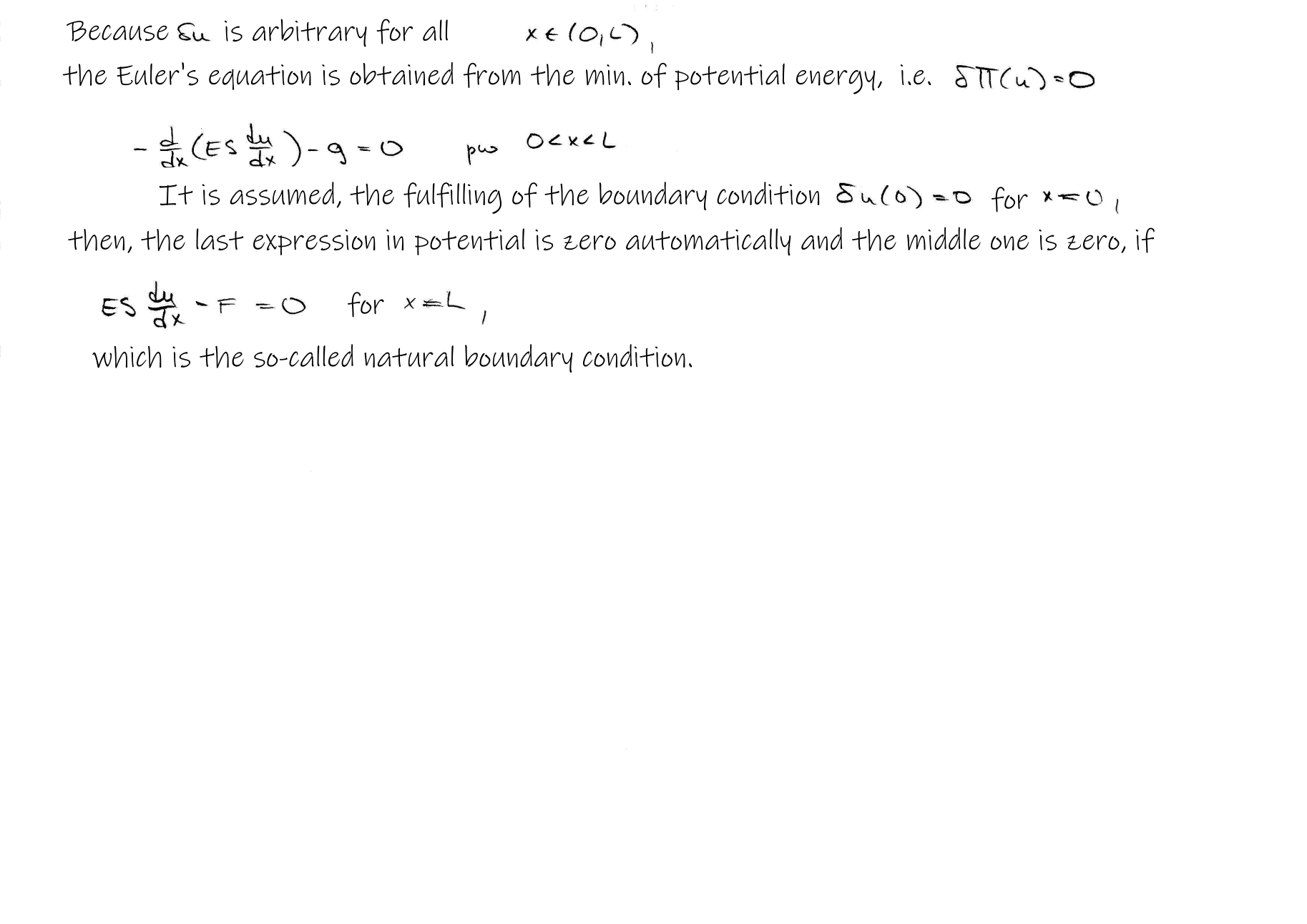
where \(L\) is the length of the bar, \(A\) is the cross-sectional area and \(E\) is the Young's modulus. The one type of boundary conditions can be prescribed at the boundary points. They can be expressed in terms of the displacements as
where \(\hat{P}\) is the prescribed external axial load.
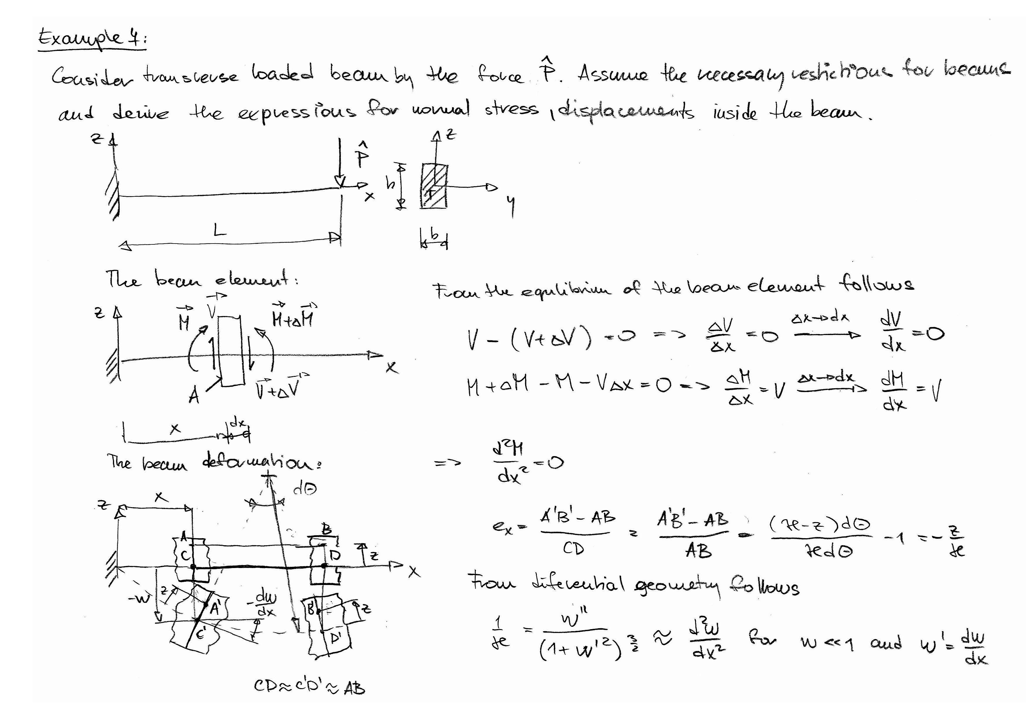
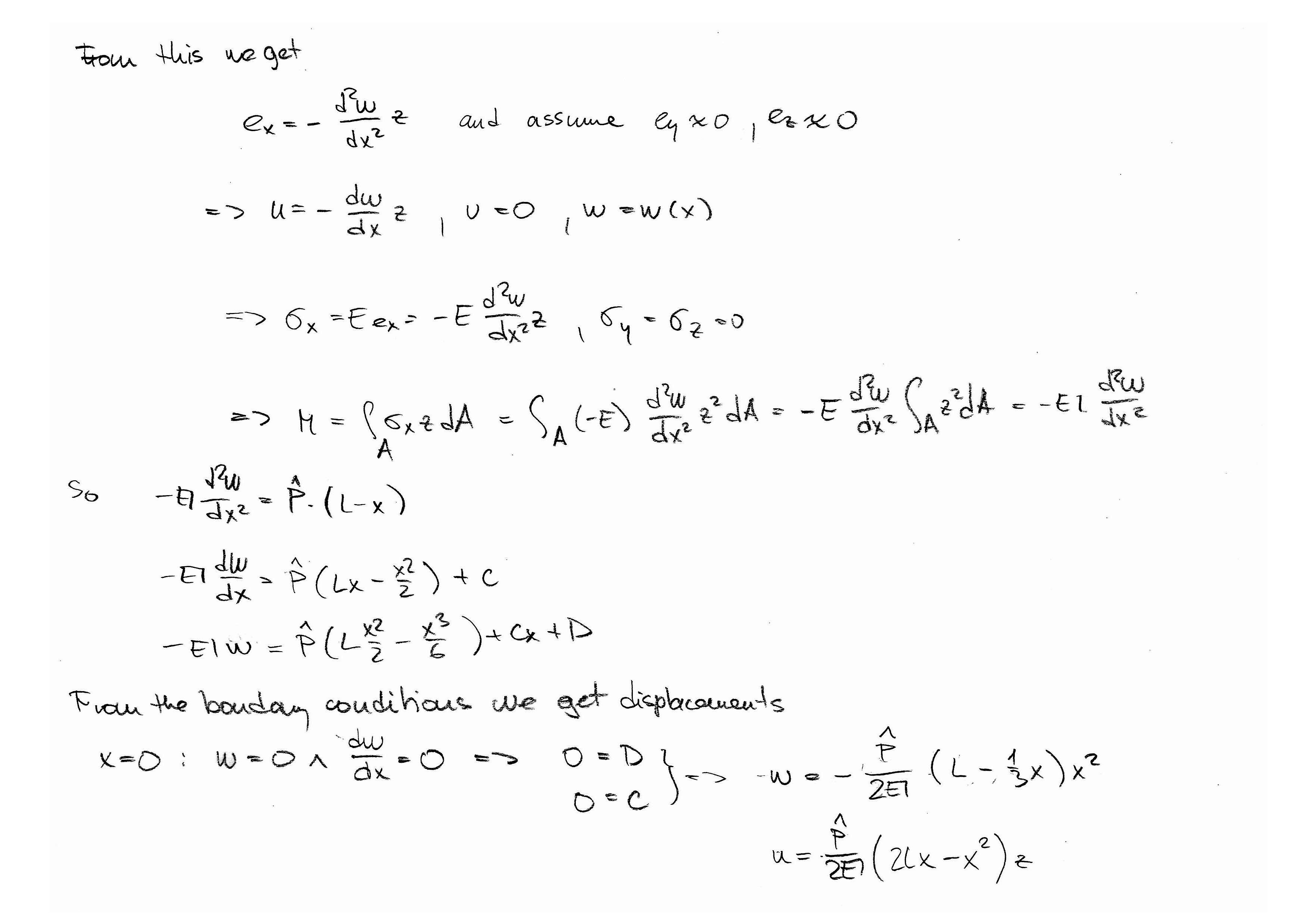
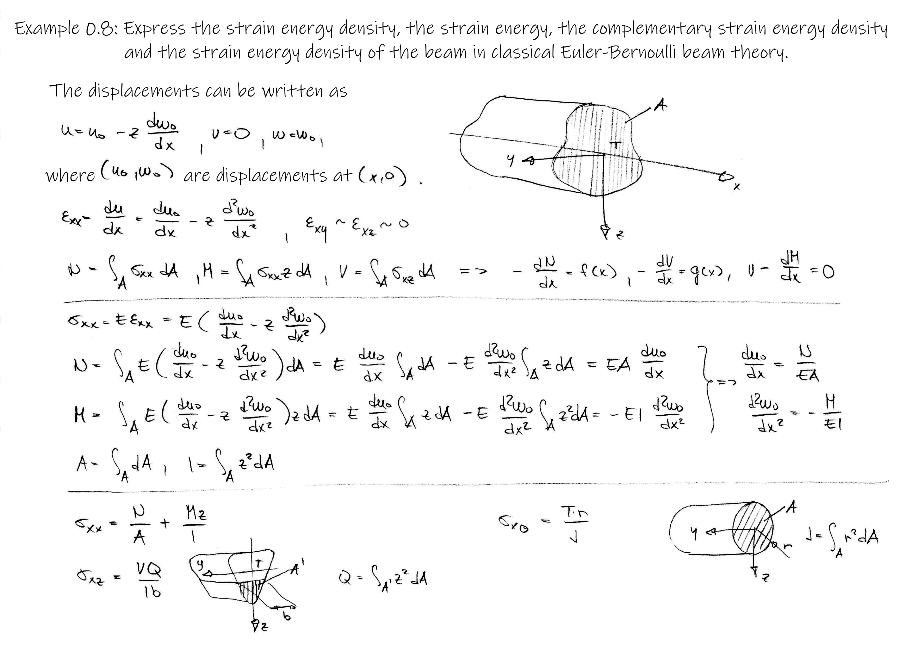
Theory of straight beams
Beams are probably the most common type of structural members. In linear analyses, the individual effects of bending, twisting, buckling and axial deformation can be superimposed. To study the bending effects alone, we place additional restrictions to the above discussed restrictions in the case of axial loaded bars. These additional restrictions on the geometry and loading of beams are as follows
The cross section of the beam has a longitudinal plane of symmetry.
The resultant of the transversely applied loads lies in the longitudinal plane of symmetry.
Plane sections originally perpendicular to the longitudinal axis of the beam remain plane and perpendicular to the longitudinal axis after bending.
In the deformed beam, the planes of cross sections have a common intersection, that is, any line originally parallel to the longitudinal axis of the beam becomes an arc of a circle.
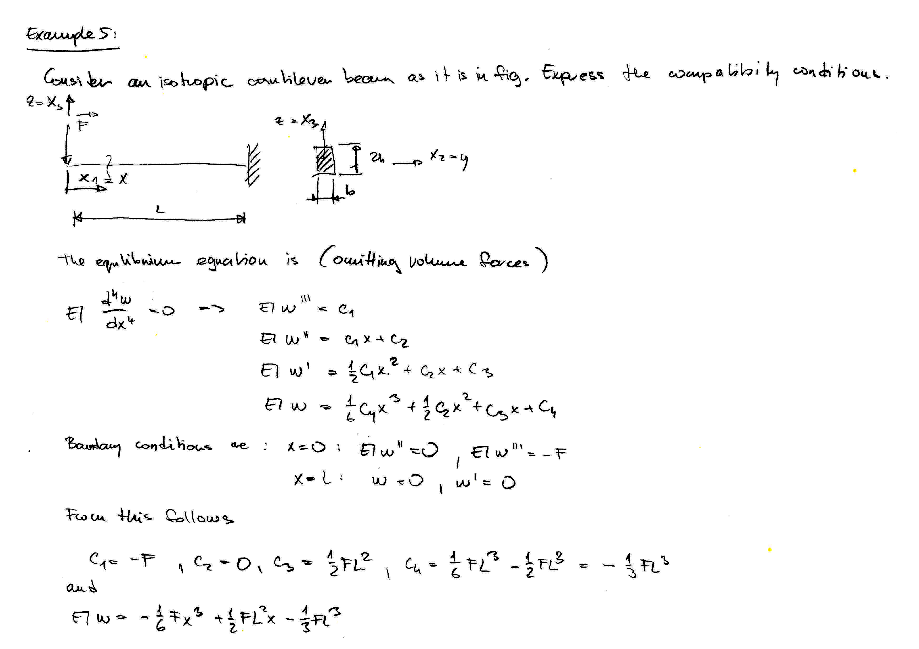
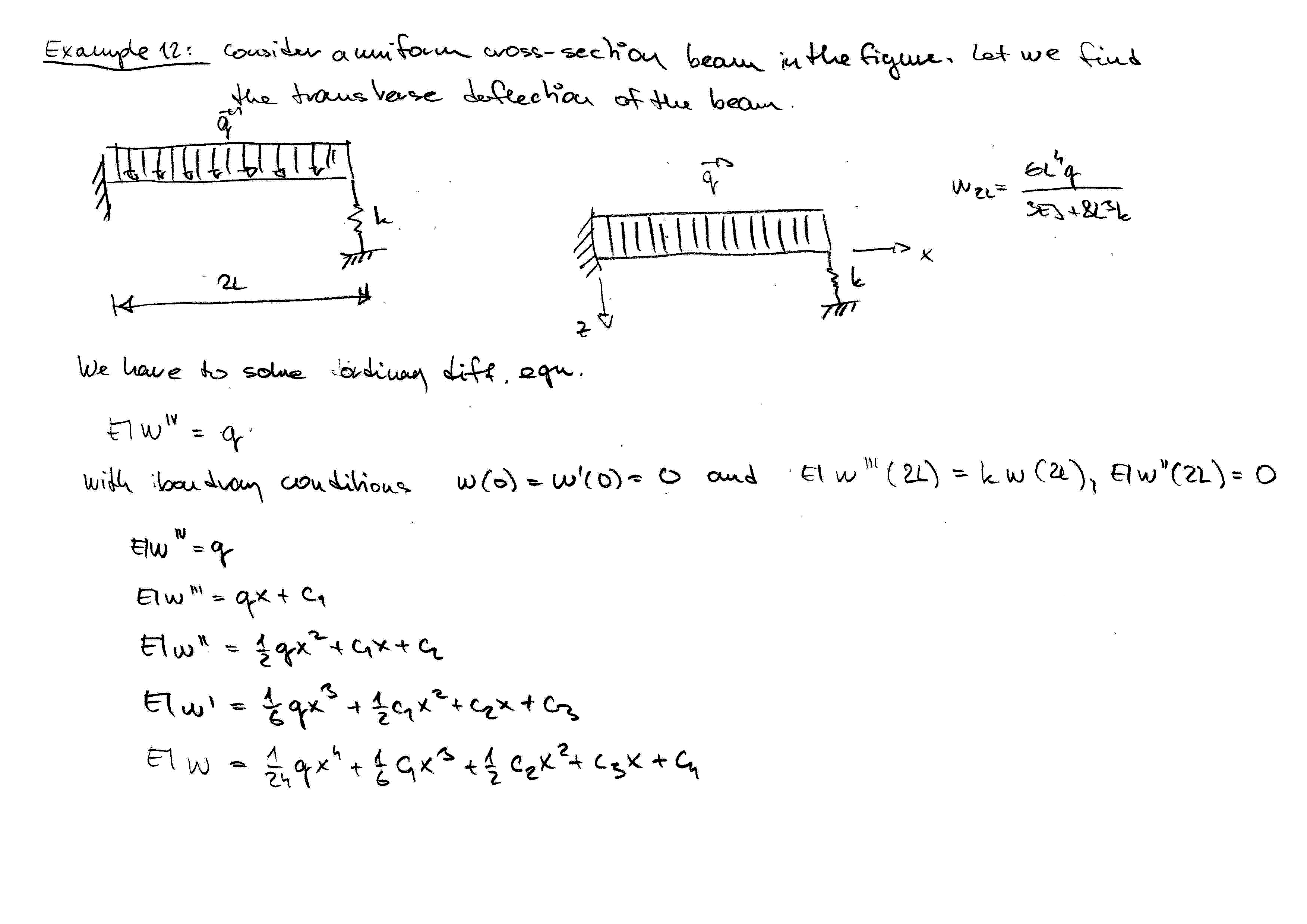
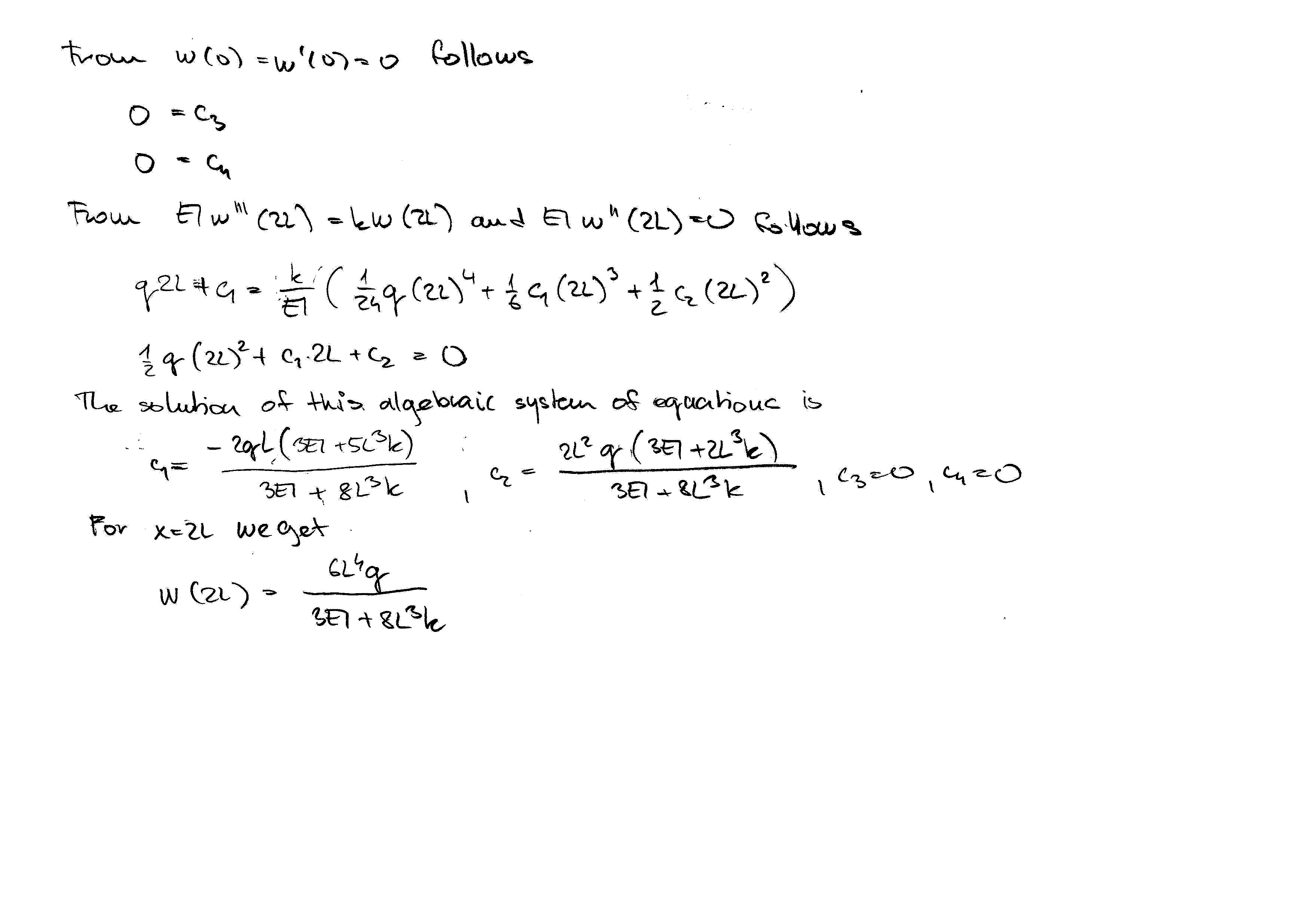
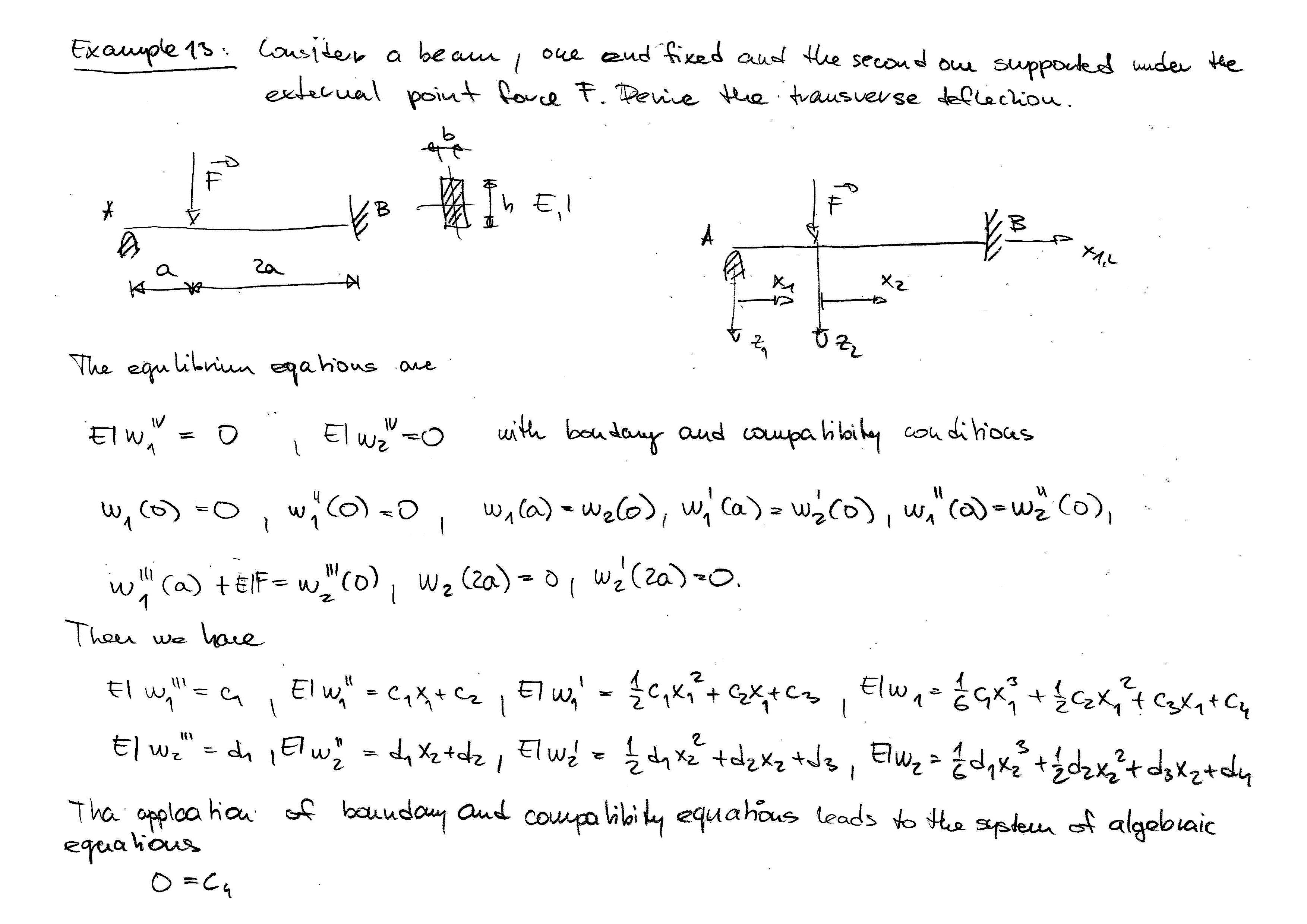
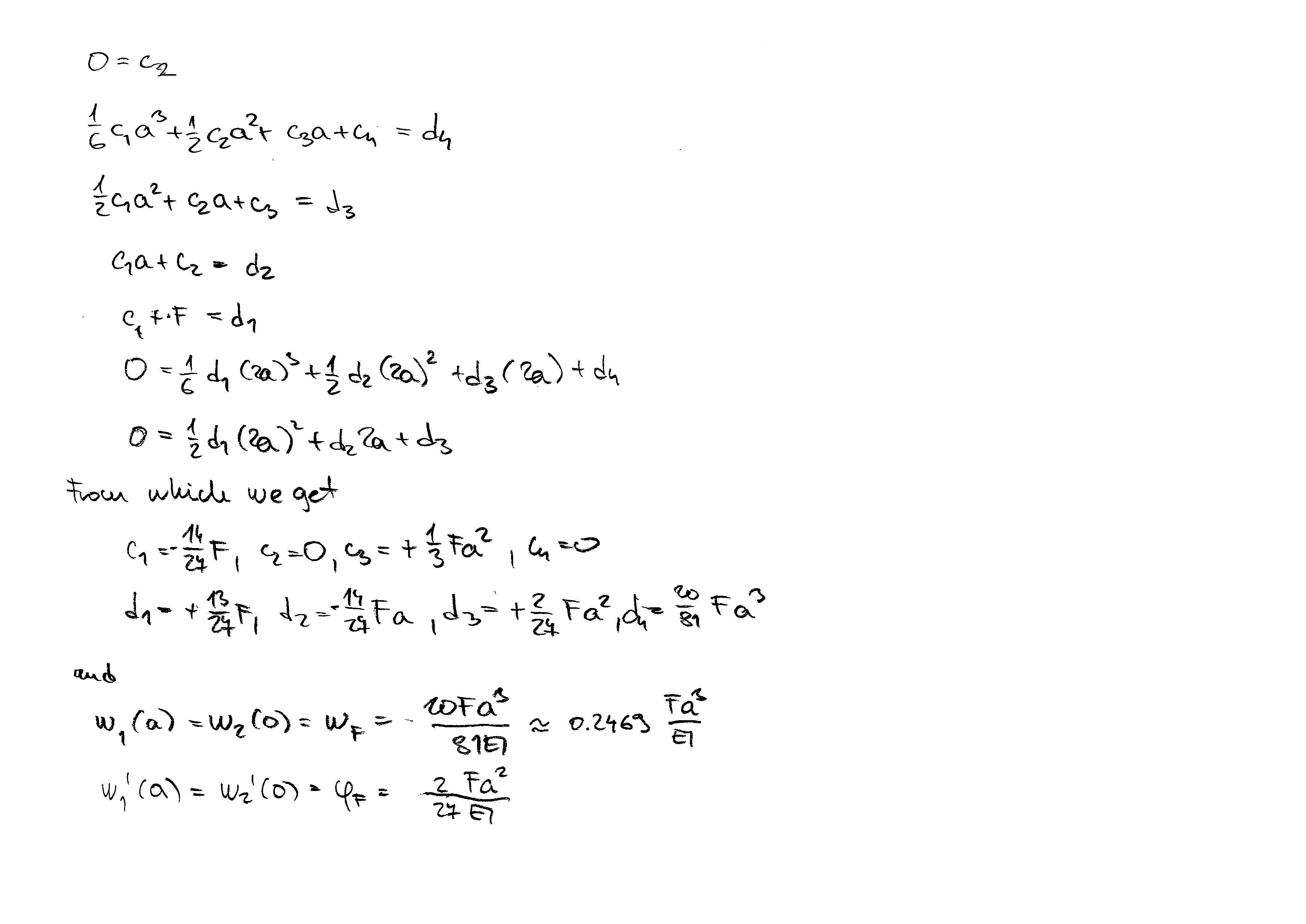
These restrictions with restriction on axial loaded beam form following mixed boundary-value problem (115) to
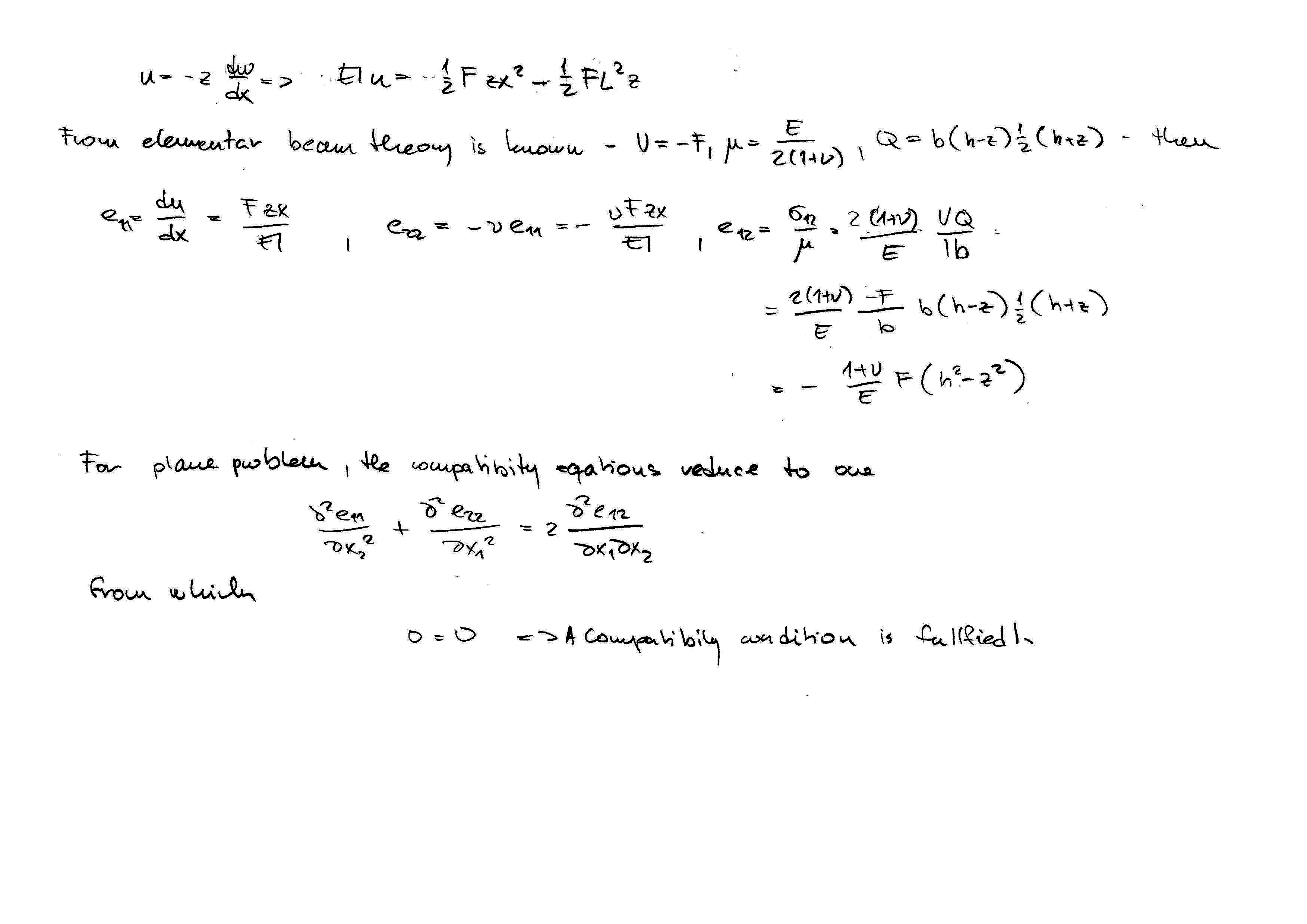
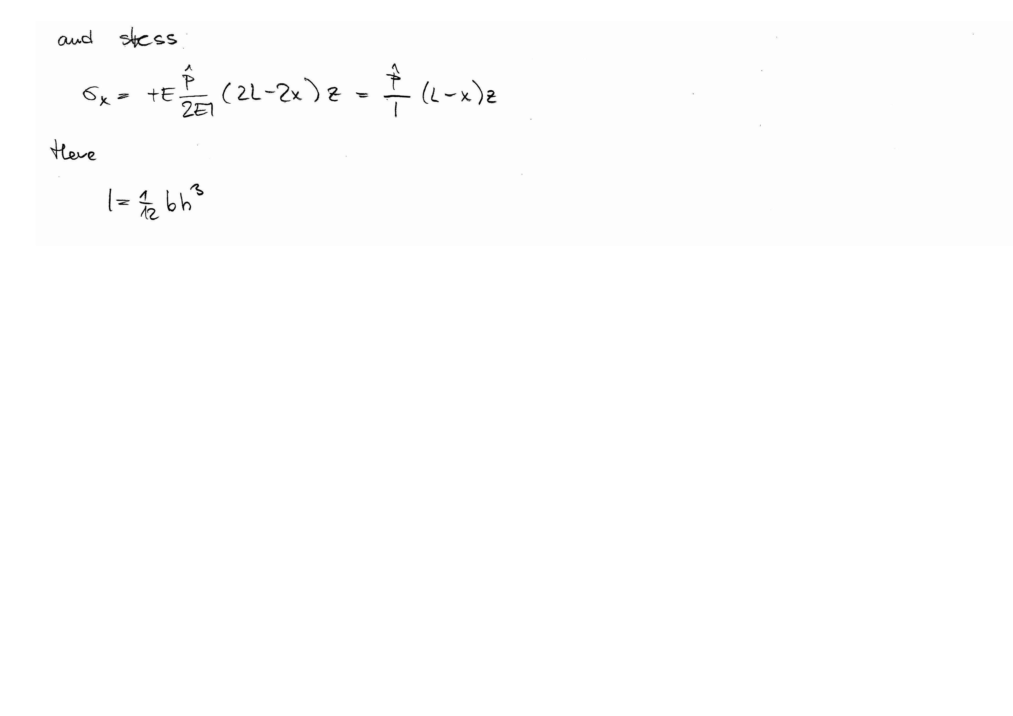
where \(L\) denotes the length of the beam, \(h\) is the width of the cross section, \(E\) is the Young`s modulus and \(I\) is the moment of inertia of the cross section about the \(y\)-axis perpendicular to the plane of beam and its external loadings, i.e. \(zx\)-plane. Internal moment \(M_y\) and shear force \(V_z\) are the resultants of the elementary moments of normal forces and tangential forces across the beam cross section
and must be in equilibrium with external volume forces
The moment \(Q_y\) of the area \(A^{\prime}\) bounded by line \(z\) and the top surface of the beam about the neutral axis is
The boundary condition specified at the ends of the beam can be
where \(\hat{w}\), \(\hat{\theta}\), \(\hat{V}\) and \(\hat{M}\) are prescribed external deflection, rotation, shear force and moment, respectively.
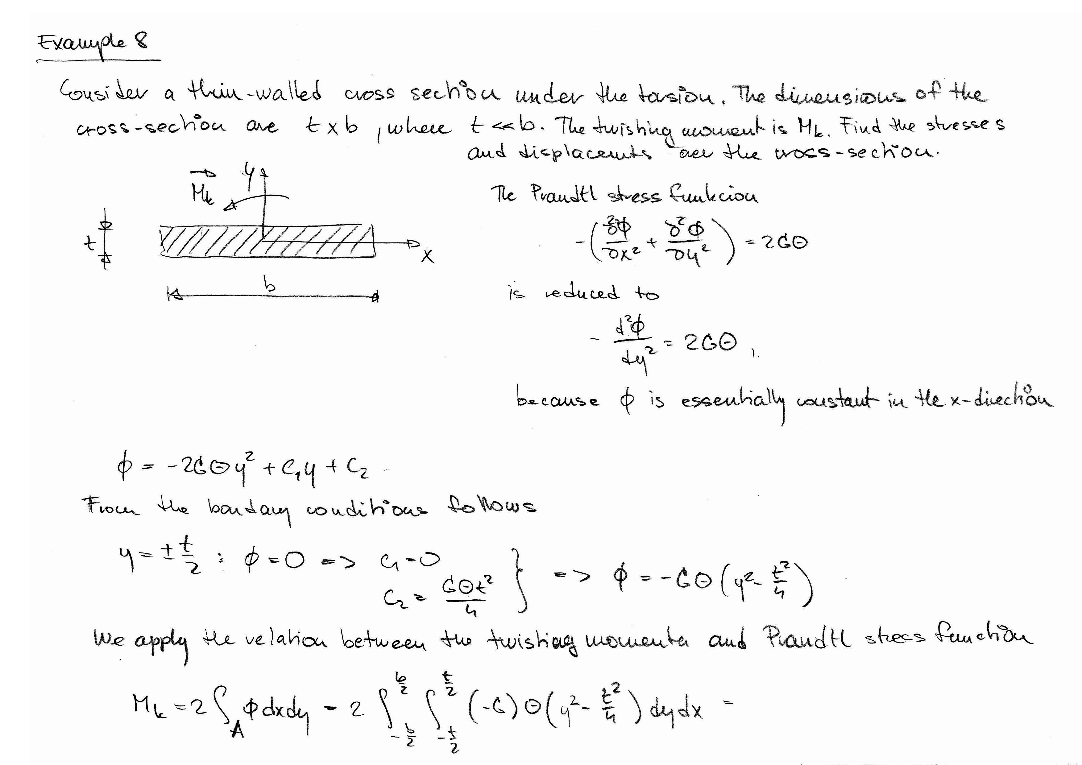
Torsion of prismatic member
The main restrictions of the torsion theory of prismatic bars are
The material is homogeneous and obeys Hook's law.
The cross section of the member is arbitrary but constant along the length.
The warping of cross section is permitted, but is taken to be independent of axial location.
The projection of any warped cross section rotates as a rigid body, and the angle of twist per unit length is constant.
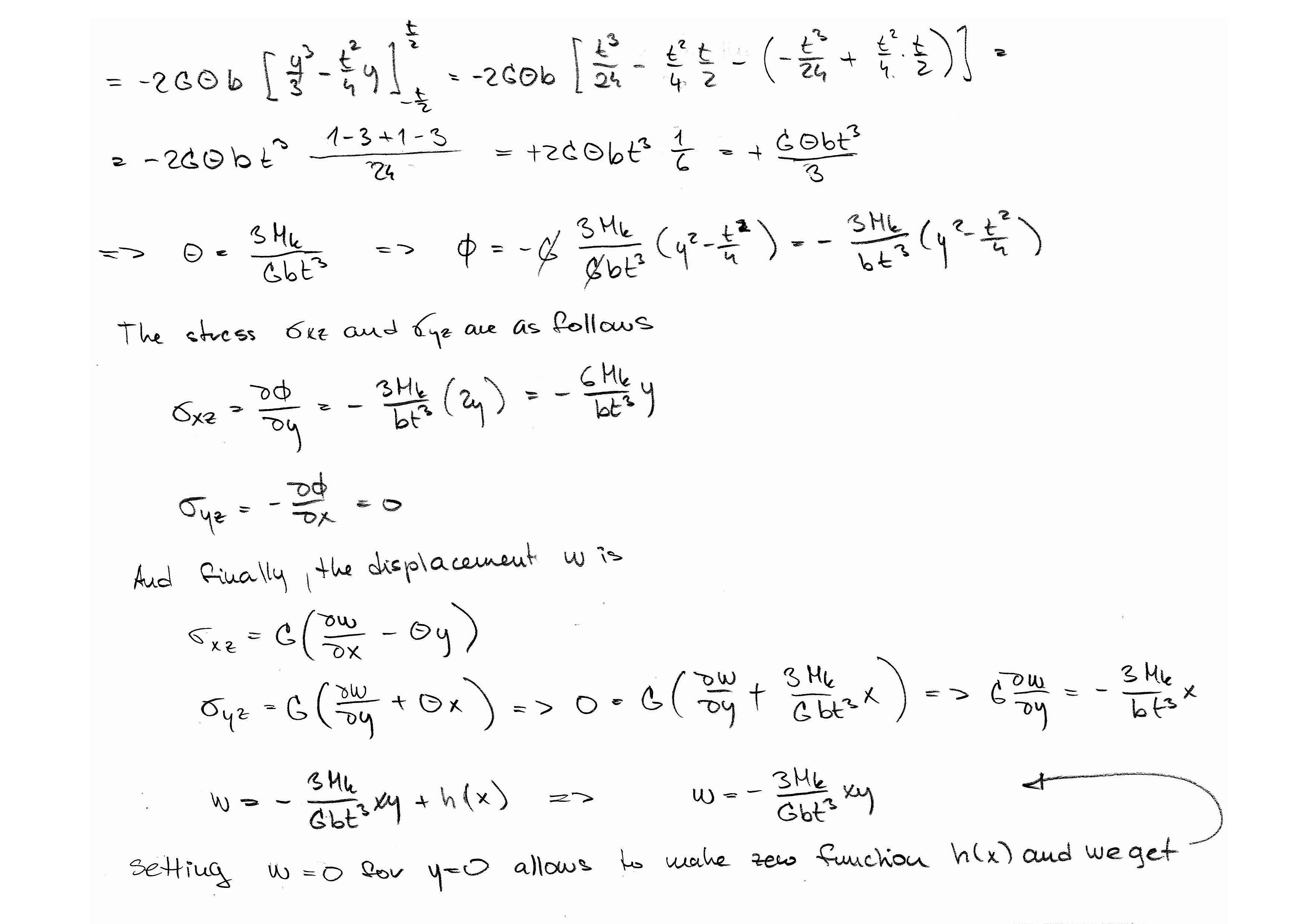
These restrictions allows one to take the form of equilibrium equation as follows
where \(A\) is the domain of the cross section, \(G\) is the shear modulus and \(\theta\) is the angle of twist and \(w\) is the warping function. The function \(\Phi(x,y)\) is known as the Prandtl stress function and it is defined as
and must obeying the boundary condition
where \(S\) is the boundary of the cross section. The applied twisting moment \(M_z\) is related to the Prandtl stress function as
Plane elasticity
Consider a linear elastic solid of uniform thickness \(h\) bounded by two parallel planes \(z=-h/2\) and \(z=h/2\) and by any closed boundary \(S\). When the thickness \(h\) is very large, the problem is considered to be a plain-strain problem, and when the thickness is small compared with the lateral dimension (\(x\), \(y\) in this case), the problem is considered to be a plane-stress problem. Both of these problems are simplifications of three-dimensional elasticity problems under the following assumptions on loading
The body forces and applied boundary forces, if any, do not have components in the thickness direction.
The body forces do not depend on the thickness coordinate, and the applied boundary forces are uniformly distributed across the thickness.
No loads are applied on the parallel planes bounding the top and bottom surfaces.
The assumption that the force are zero on the parallel planes implies that the stresses associated with the \(z\)-direction are negligibly small for plane stress problems
For plane-strain problems, the assumption is that the strains associated with the \(z\)-direction are zero (in generalized plane-strain problems, they are assumed to be constant)
An example that illustrates the difference between plane-stress and plane-strain problems is provided by the bending of a rectangular cross-section beam. If the beam is narrow, it is considered a plane-stress problem. If the beam is very wide, it is considered a plane-strain problem. The equations governing the two types of plane elasticity problem discussed above can be obtained from the three-dimensional equations by using the assumptions (146) and (147)
with the constitutive equations
for \((x,y)\in R\), \(R\) is the plane domain and \(f_x\) and \(f_y\) are coordinates of body forces. The strain-displacement relations are reduced to
The elasticity constants for orthotropic material in (149) are given as follows
or
where \(E_1\) and \(E_2\) are Young's moduli in one and two material directions, \(\nu_{ij}\) is Poisson's ratio for transverse strain in the \(j\)-th direction when stressed in the \(i\)-th direction, and \(G_{12}\) is the shear moduli in the 1-2 plane. For isotropic material we have
The natural and essential boundary conditions are as follows
and
where \(\boldsymbol{n}=(n_x,n_y)\) denotes unit normal to the boundary \(S\), \(S_1\) and \(S_2\) are disjunct portions of the boundary \(S\), \(\hat{\boldsymbol{t}}=(\hat{t}_x,\hat{t}_y)\) denotes specified boundary force and \(\hat{\boldsymbol{u}}=(\hat{u},\hat{v})\) denotes specified boundary displacement.
Lecture 8
Work and Energy
If \(\boldsymbol{F}=\boldsymbol{F}(\boldsymbol{x})\) is the distributed force acting on a particle occupying position \(\boldsymbol{x}\) in the body and \(\boldsymbol{u}=\boldsymbol{u}(\boldsymbol{x})\) is the displacement of the particle, then the work done on the particle is \(\boldsymbol{F}\cdot\boldsymbol{u}\), and the total work done on the body is the sum of work done on all particles of the body
where \(\Omega\) denotes the volume of the body. If a body is subjected to point forces \(\boldsymbol{F}_1\), \(\boldsymbol{F}_2\), etc. that displace the points of action by displacements \(\boldsymbol{u}_1\), \(\boldsymbol{u}_2\), etc., respectively, then the work done by the forces on the body is the sum of the work done by individual forces
Note that in this case, \(\boldsymbol{F}_i\) and \(\boldsymbol{u}_i\) are not vector functions but constant vectors. Similarly can be obtained for moments \(\boldsymbol{M}_i\) and angles \(\boldsymbol{\theta}_i\)
Energy is the capacity to do work. It is a measure of the capacity of all forces that can be associated with matter to perform work. Work is performed on a body through a change in energy. The energy \(E\) of a body acted upon by time-dependent forces \(\boldsymbol{F}=\boldsymbol{F}(\boldsymbol{x},t)\) is given by the expression
Both work and energy are scalars that are independent of the coordinate system used to express them. The choice of the coordinate system only dictates the components of force and displacement, but their product is the same in any coordinate system.
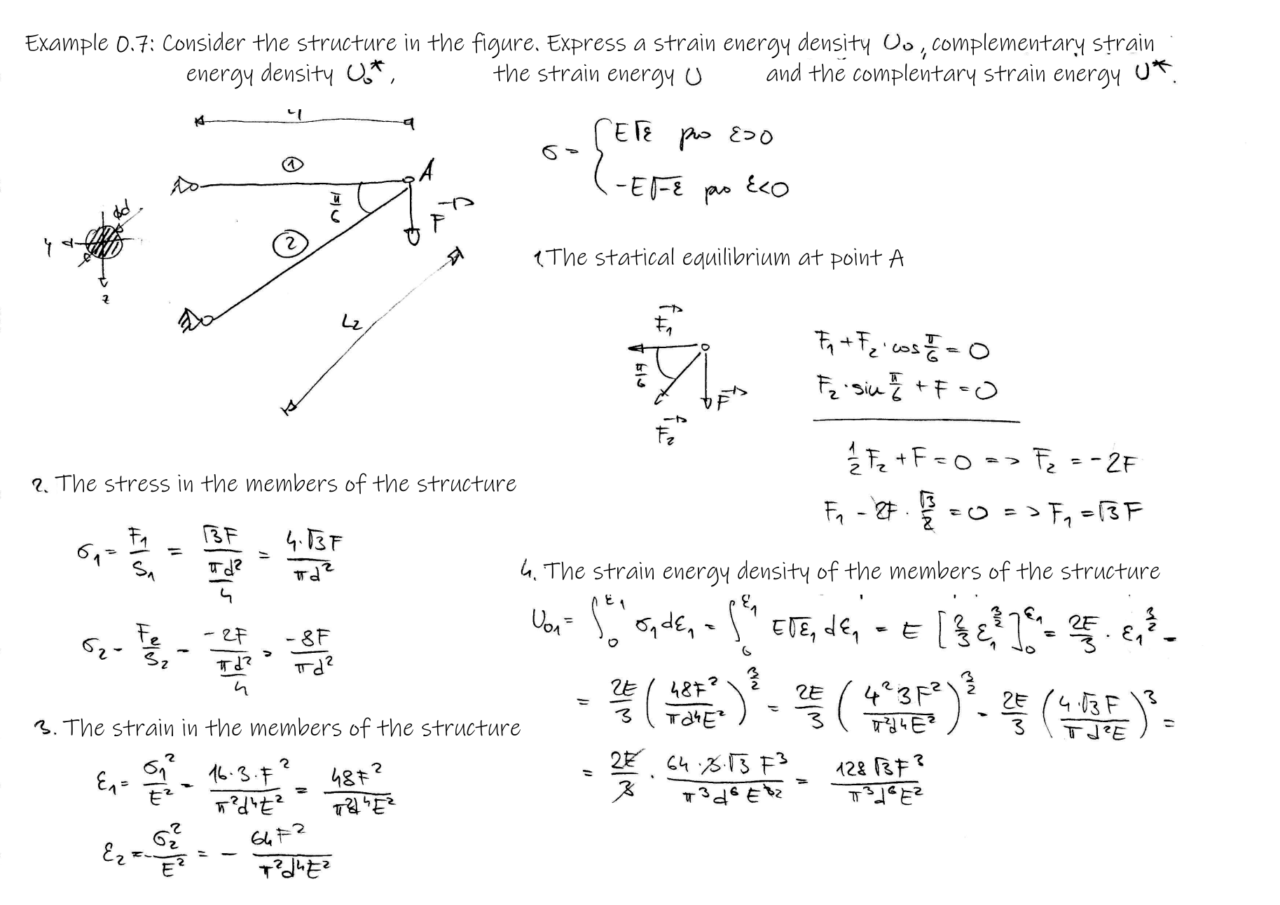
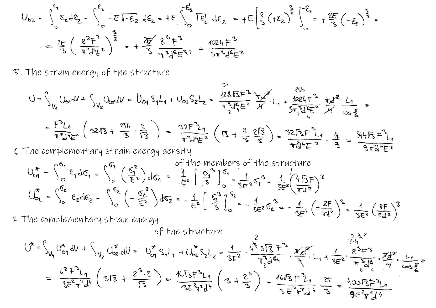
Strain Energy and Complementary Strain Energy
The stress components \(\sigma_{ij}\) can be evaluated from the strain energy density function \(U_0\) under the conditions, that it is independent of the temperature \(T\) and the loading process of the body is isothermal, as it was shown in section Deformations Due to Temperature Change and Thermoelastic Constitutive Equations. The existence of a scalar function \(U_0=U_0(e_{ij})\) depending on strains only, from which the stresses are derivable, is of special importance. Such stresses satisfy the energy equation and they are said to be conservative. Hence, under the isothermal conditions, we have
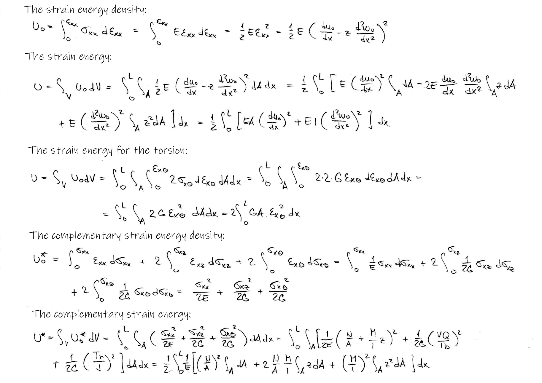
The strain energy density \(U_0\) is given by integrating (161)
This expression is valid for all elastic bodies with linear or nonlinear strain-displacement relations. The complement to the strain energy density \(U_0\) with respect to the double-dot product \(\sigma_{ij}e_{ij}\) is the so-called complementary strain energy density, \(U_0^*\), which can be computed from
For linear elastic materials, we have
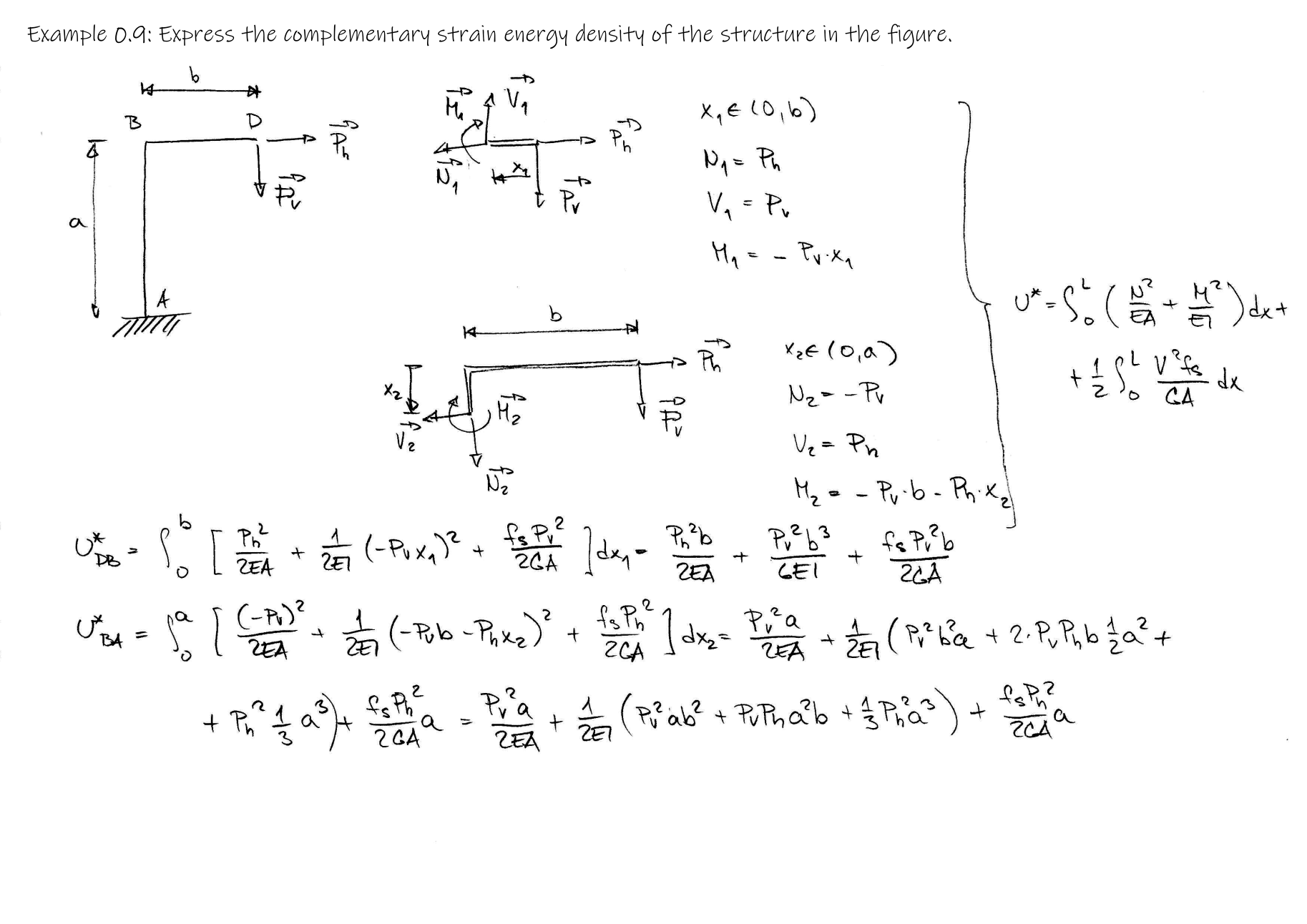
and \(U_0=U_0^*\). The strain energy \(U\) and complementary strain energy \(U^*\) of an elastic body are given by
Analogous to (161), the strains are computed from
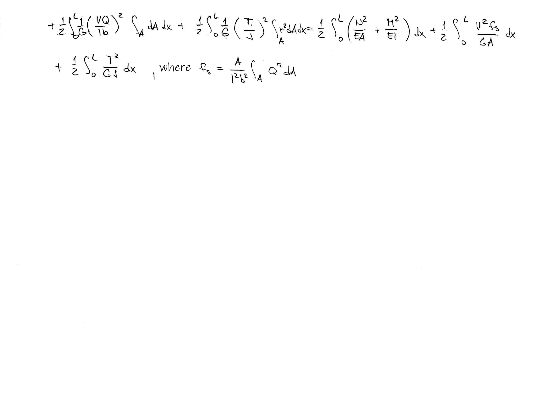
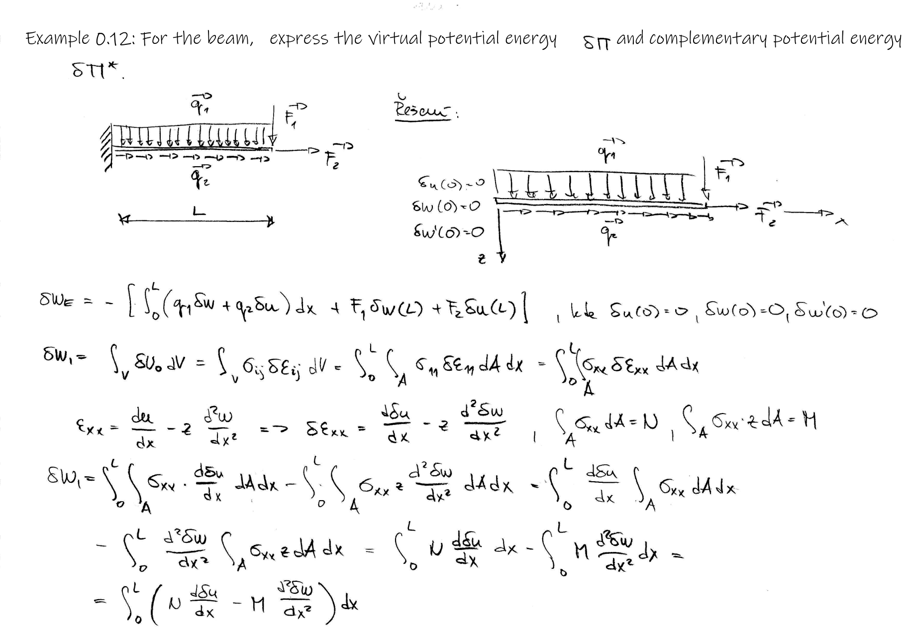
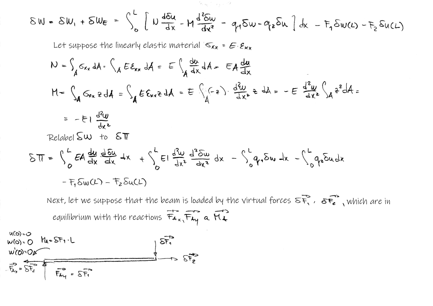
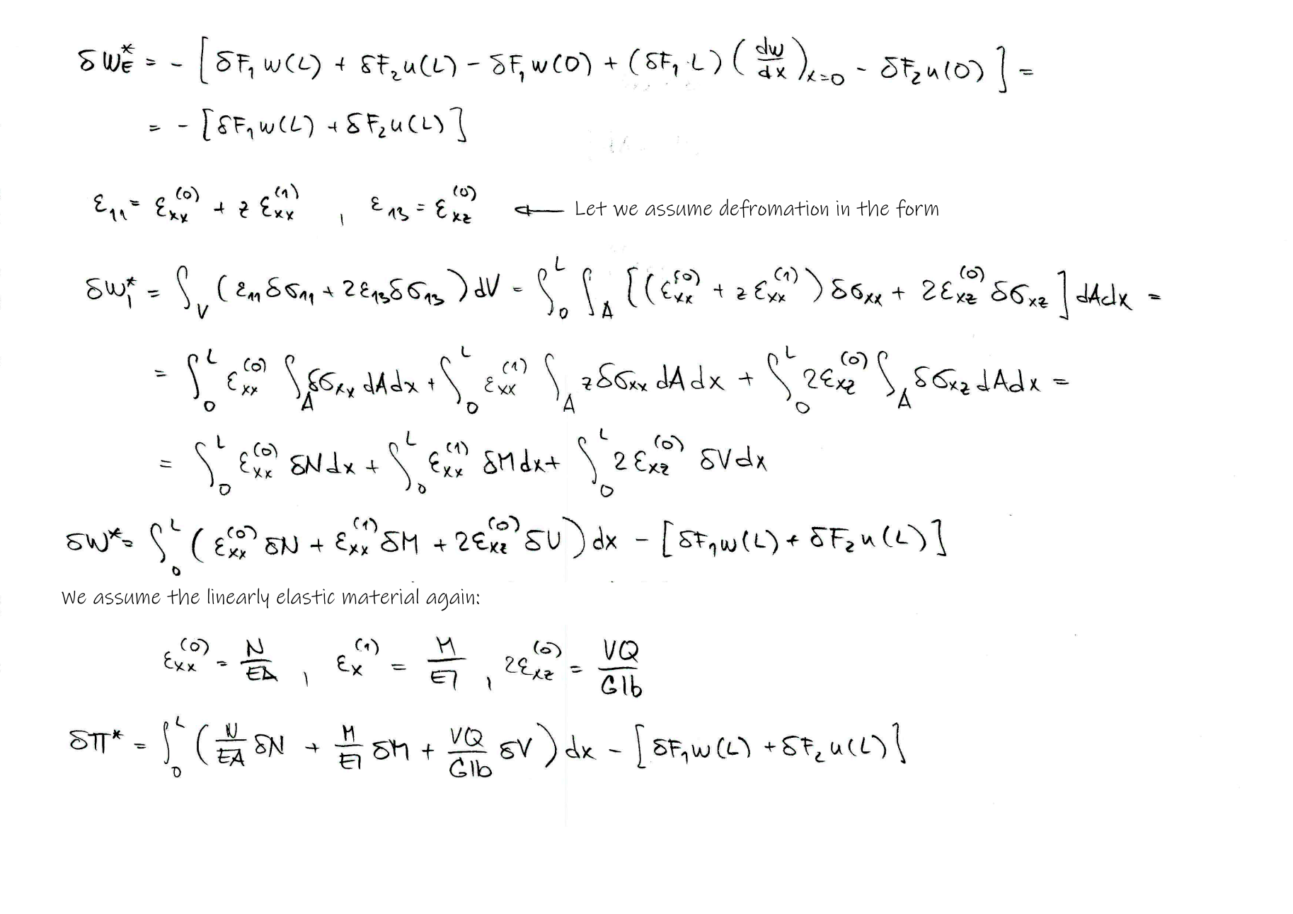
It should be noted, that both the strain energy density \(U_0\) and complementary energy density \(U^*_0\) can be expressed either in terms of displacements or in terms of forces. The expressions for strain energy \(U\) and complementary energy \(U^*\) of a beam experiencing bending moment \(M_y=M_y(x)\), axial force \(N=N(x)\), transverse displacement \(w\) and axial displacement \(u\), but neglecting the shear forces \(V_z=V_z(x)\), are as follows
Hamilton's principle
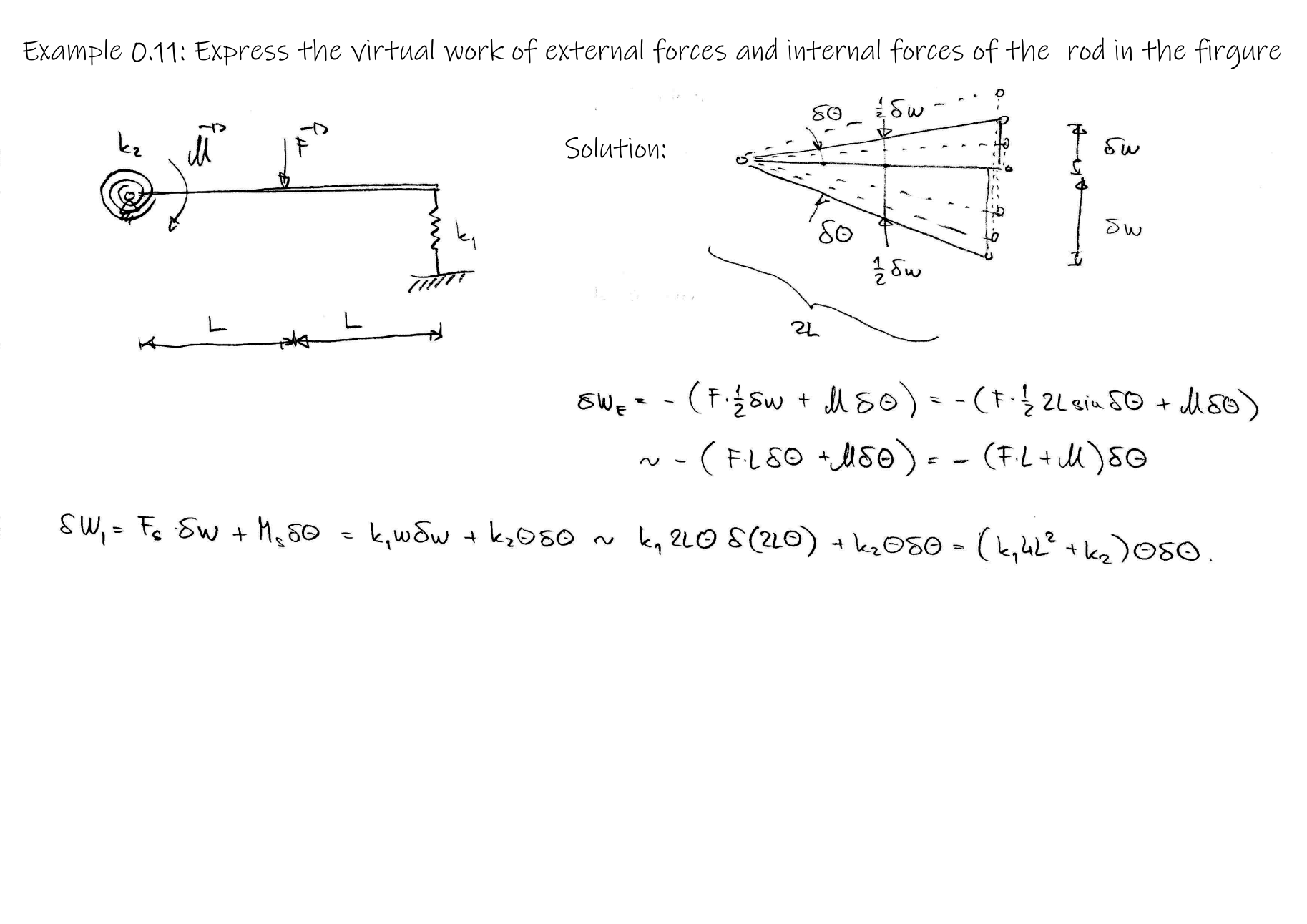
The work done on the body at time \(t\) by the resultant force in moving through the virtual displacement \(\delta\boldsymbol{u}\) is given by the expression
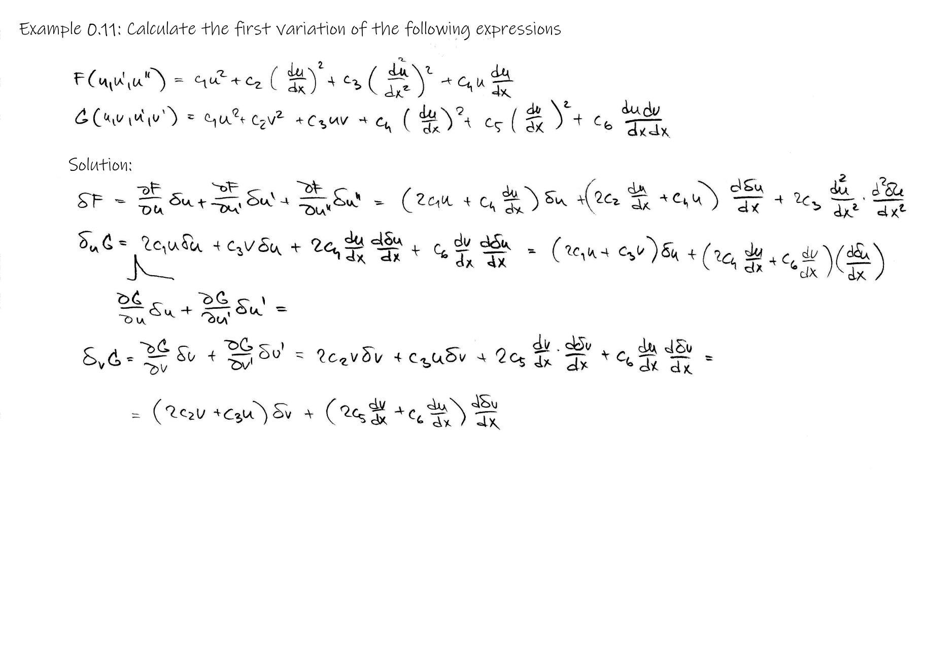
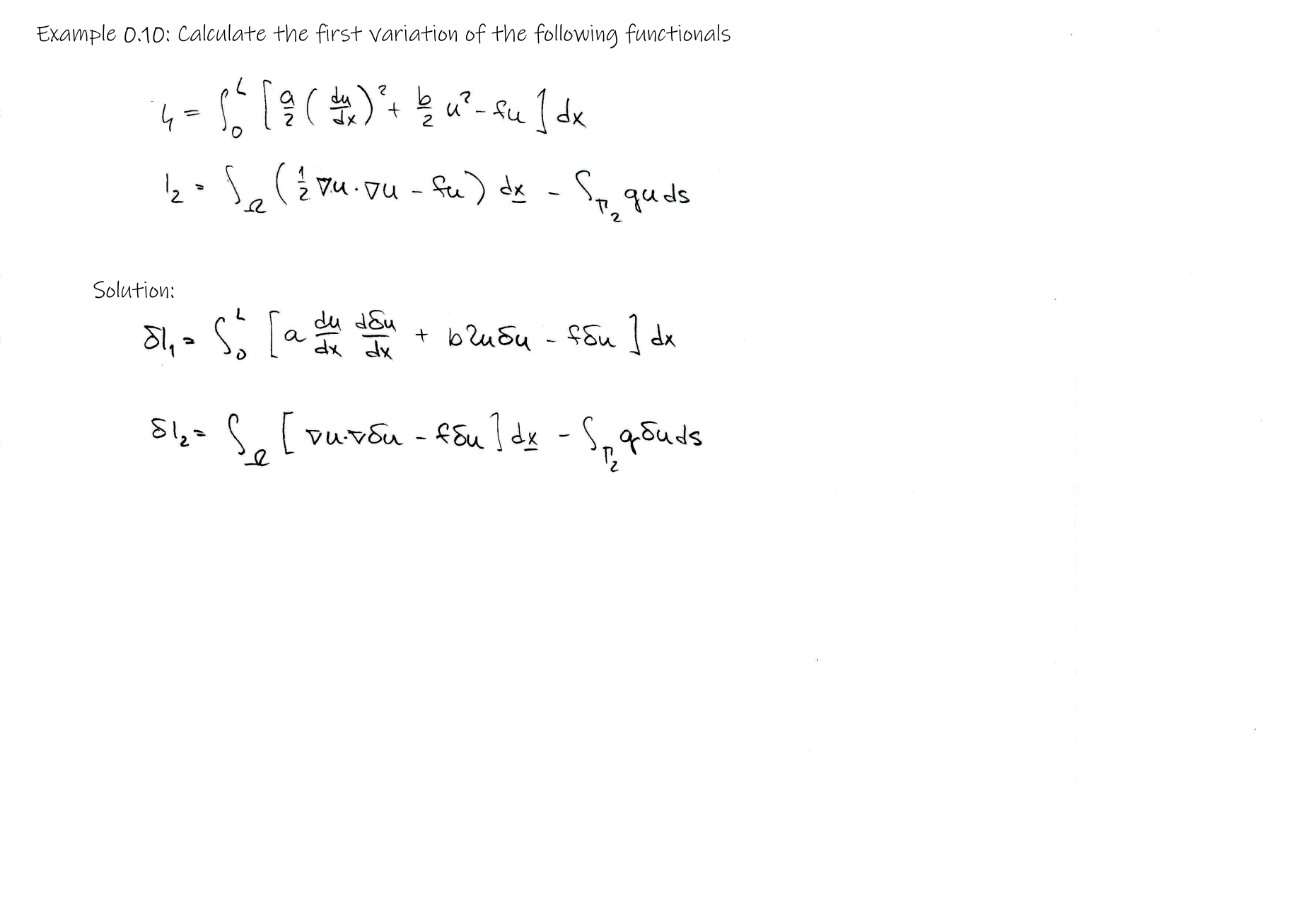
where \(f\) is the body force vector, \(\hat{\boldsymbol{t}}\) is the specified surface stress vector acting on the subdomain \(S_2\) of the boundary \(S\), and \(\boldsymbol{\sigma}\) and \(\boldsymbol{e}\) are the stress and strain tensors. The symbol \(\delta\) means variation of the displacements \(\delta\boldsymbol{u}\) and strains \(\delta\boldsymbol{e}\). It is treated the same as the differential, i.e. for displacements \(\boldsymbol{u}\) and \(\boldsymbol{v}\) we have
but unlike the differential, no restrictions to the quality are required on \(\boldsymbol{u}=\boldsymbol{u}(\boldsymbol{x})\) or \(\boldsymbol{v}=\boldsymbol{v}(\boldsymbol{x})\) as the functions of the position \(\boldsymbol{x}\). The variation \(\delta\boldsymbol{u}\) or \(\delta\boldsymbol{e}\) means the virtual displacements or virtual strains, respectively, which represent any admissible displacements or deformations of the body at the point \(\boldsymbol{x}\) under the conditions that the geometric constrains of the system are not violated and all forces are fixed at their actual equilibrium values.
The last term in (169) represents the virtual work of internal forces stored in the body (as the consequence, it is negative). The strains \(\delta\boldsymbol{e}\) are assumed to be compatible in the sense that the strain-displacement relations (40) are satisfied. The work done by the inertia force \(m\boldsymbol{a}\) in moving through the virtual displacement \(\delta\boldsymbol{u}\) is given by
where \(\rho\) is the mass density (can be a function of position) of the medium. We have from the Newton's law of motion for continuous body
the following relation
Integrating the last term in (173) by parts
considering \(\delta\boldsymbol{u}(t_1)=\delta\boldsymbol{u}(t_2)=0\), the forces \(\boldsymbol{f}\) and \(\hat{\boldsymbol{t}}\) to be conservative and that the strain energy density function \(U_0\) exists, then the general form of Hamilton's principle for a continuous medium is obtained
where \(L\) is the Lagrangian
and \(K\), \(V\) and \(U\) are the kinetic energy, potential energy of external forces and strain energy, respectively, given by the equations
The sum \(V\) and \(U\) is called the total potential energy \(\Pi\) of the body
and the Lagrangian can be written in the form
On the other hand, integration of the third term in (173) by parts and applying the divergence theorem, i.e.
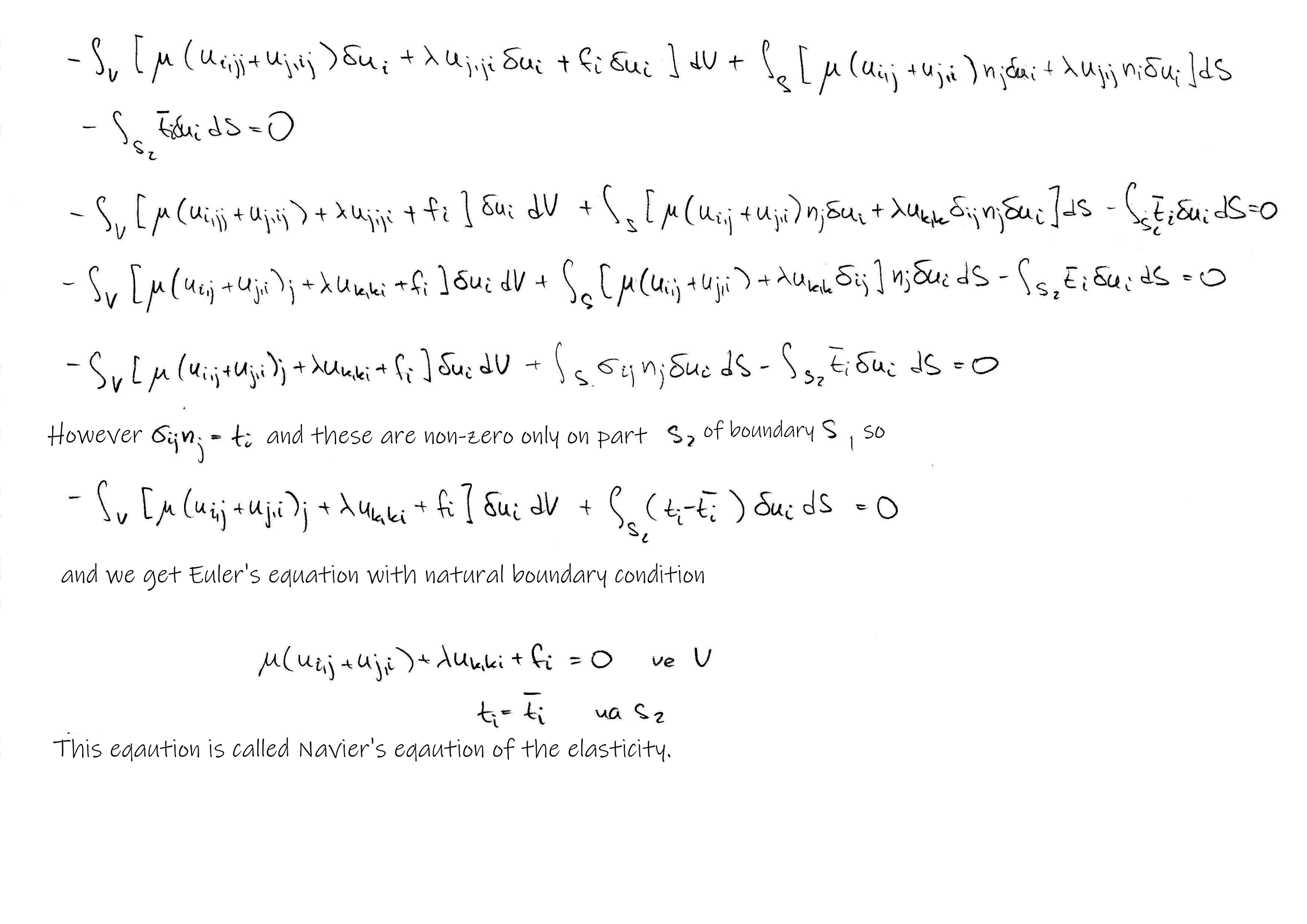
leads to the so-called Euler-Lagrange equations associated with the Lagrangian \(L\) such that
Because \(\delta\boldsymbol{u}\) is arbitrary for \(t\in(t_1,t_2)\), for \(\boldsymbol{x}\) in \(\Omega\) and also on \(S_2\), it follows that
Equations (182) are the Euler-Lagrange equations of elastic body.
Lecture 9
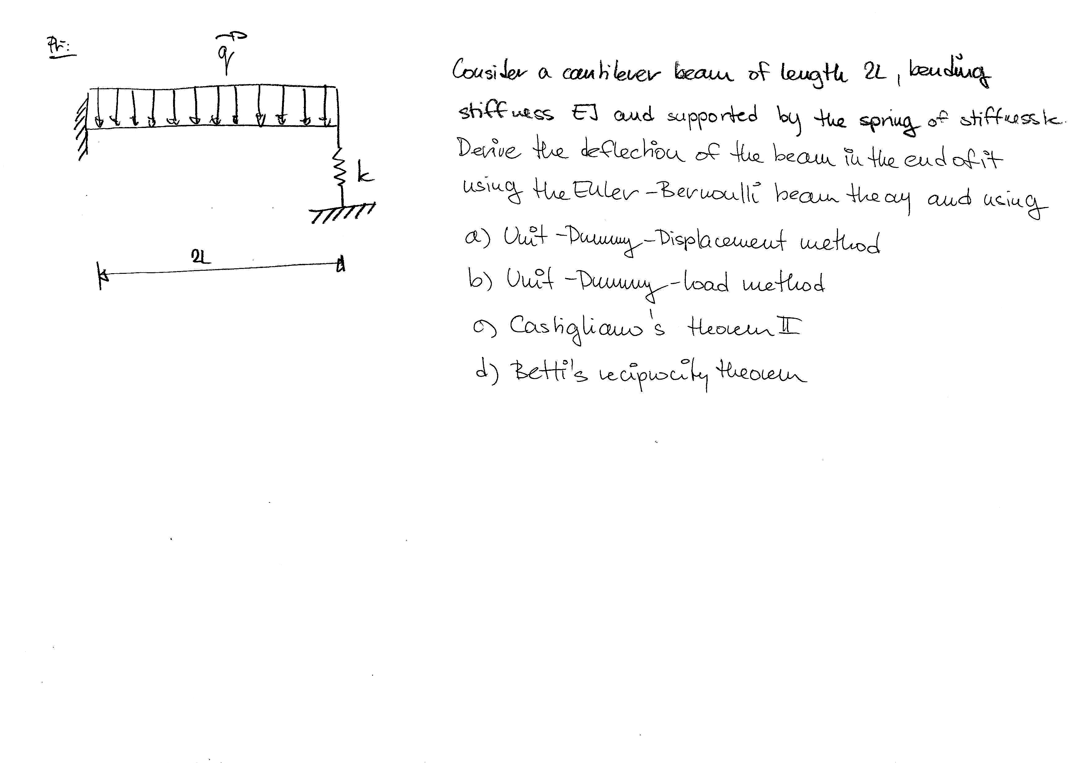
Hamilton's principle is the most general and basic principle of mechanics, from which the Euler-Lagrange equations and other laws of mechanics, as well as continuum mechanics, simply follow. The body involving no motion or forces applied sufficiently slowly that the motion is independent of time and the inertia forces are negligible is considered in the following. A wide range of continuum mechanics problems can be formulated so that this condition is satisfied. The assumption of time-independent motion also allows us to introduce several important variational methods capable of finding solutions to fairly general continuum mechanics problems.
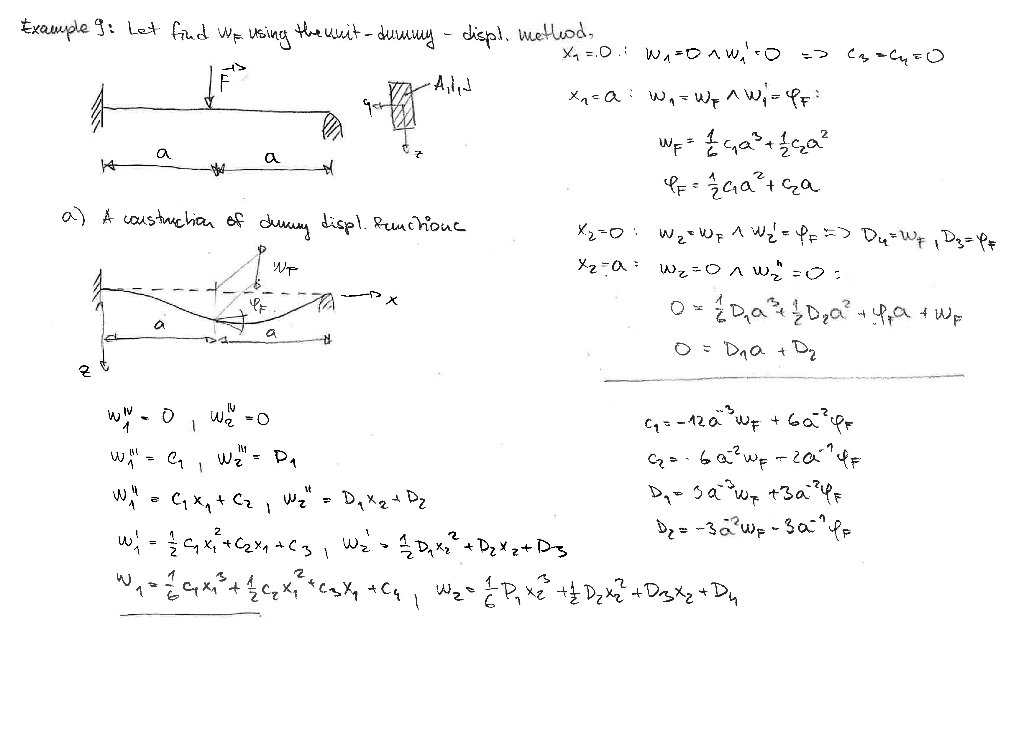
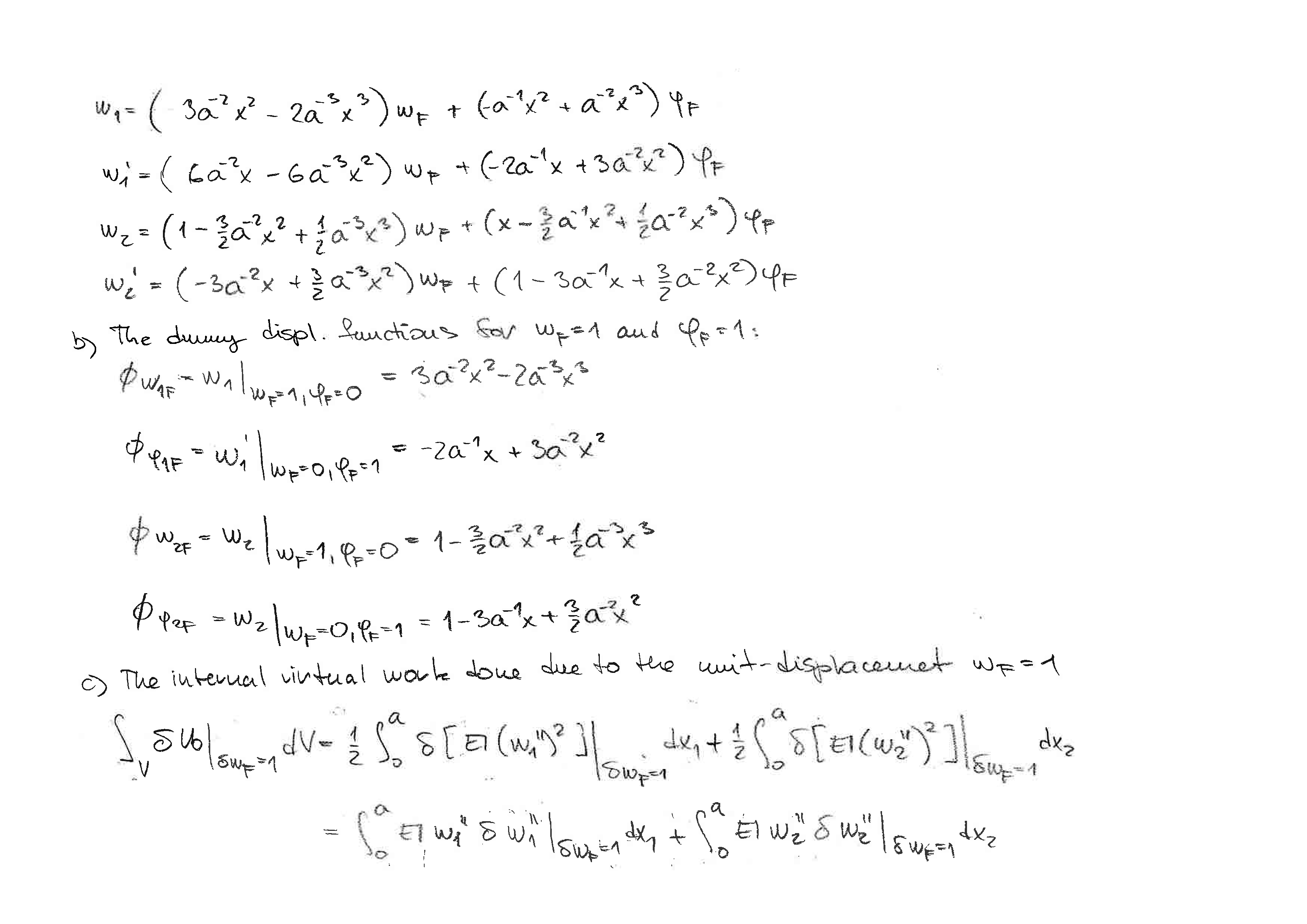
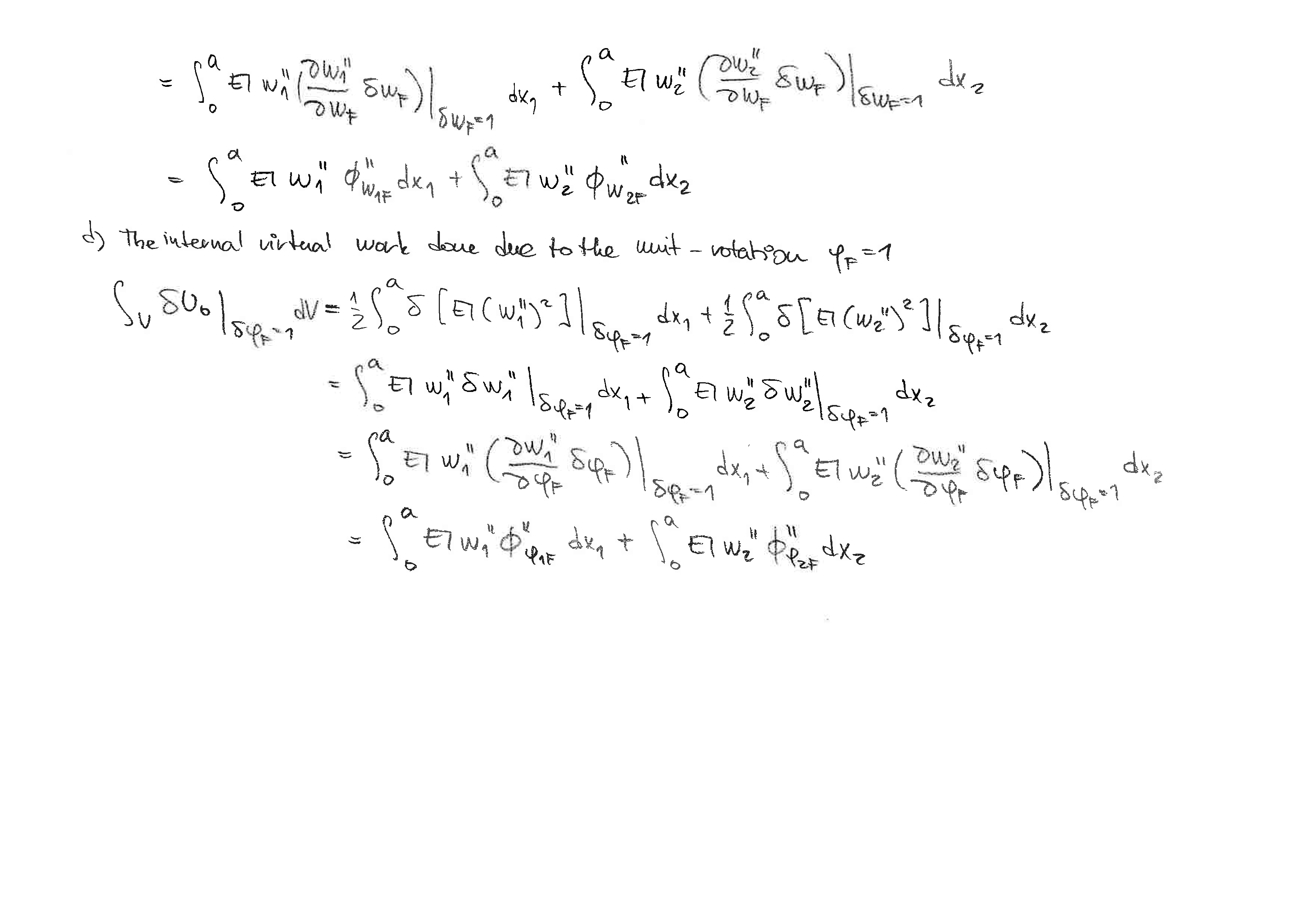
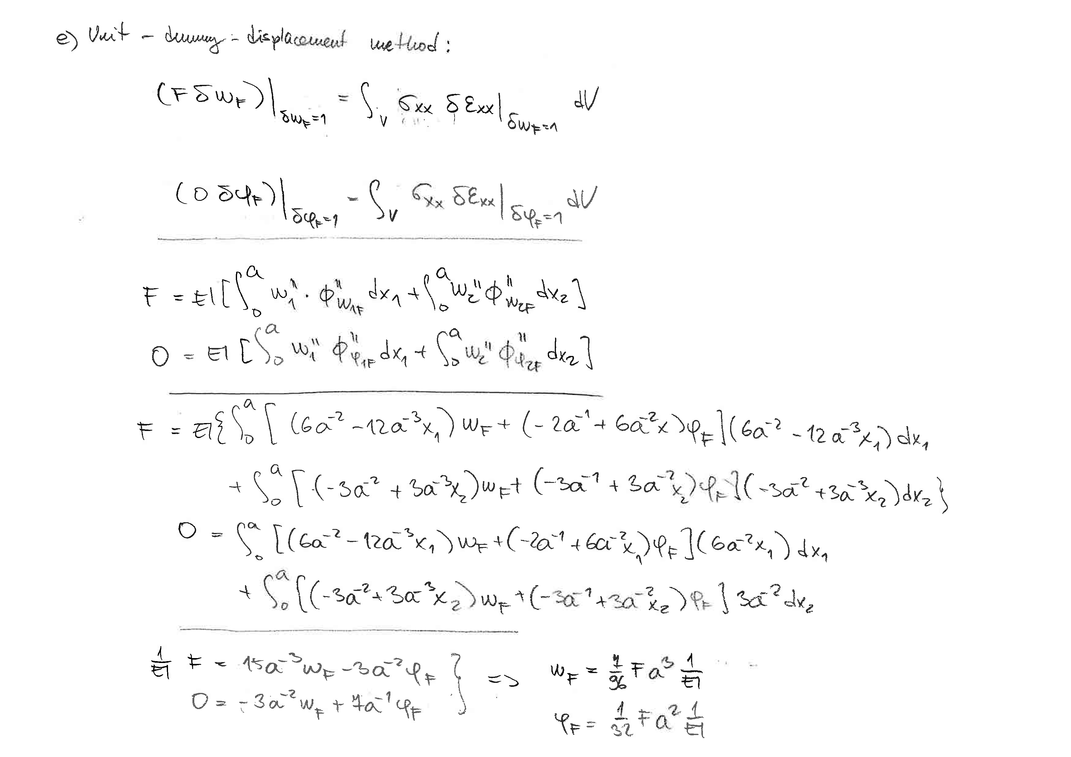
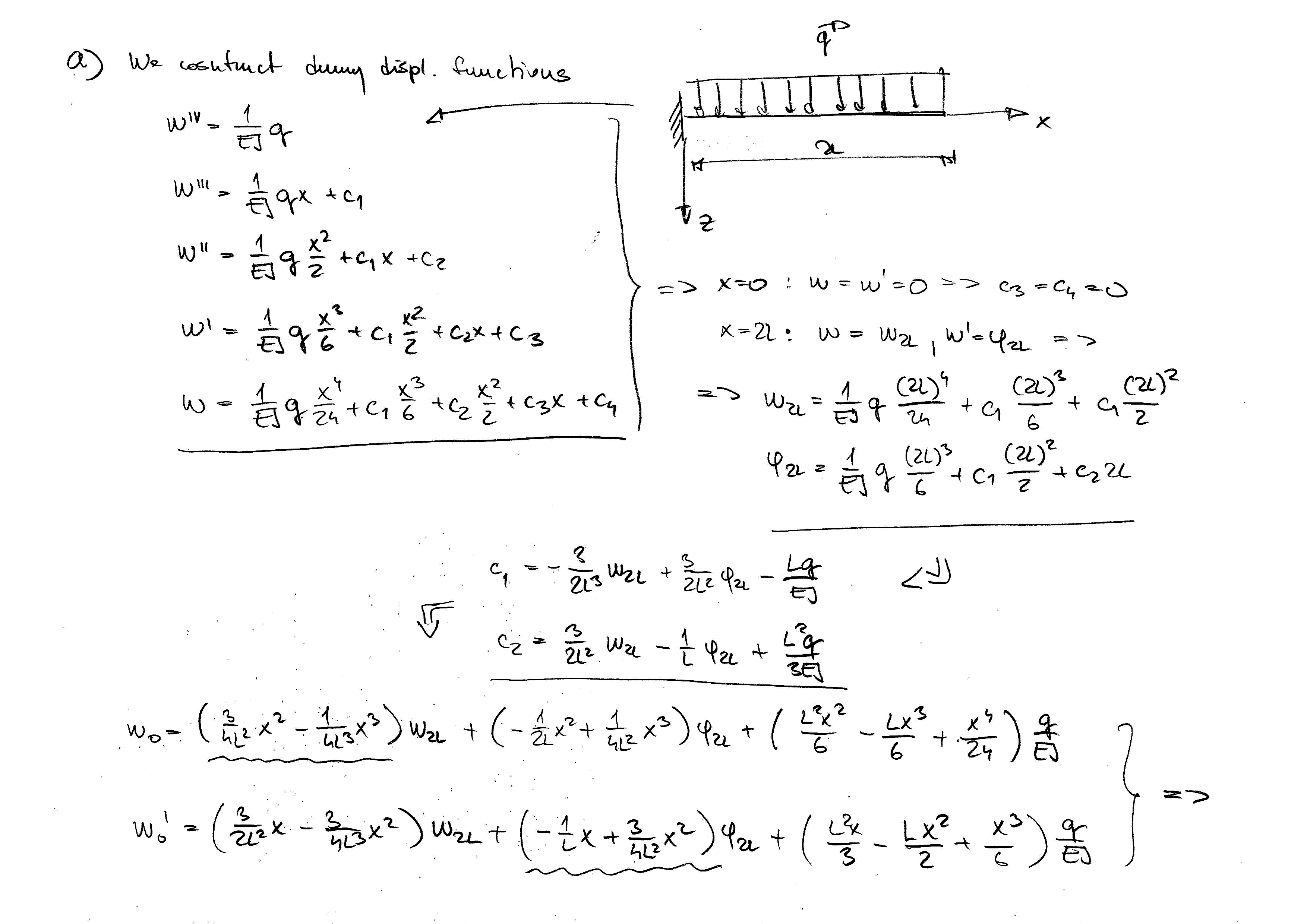
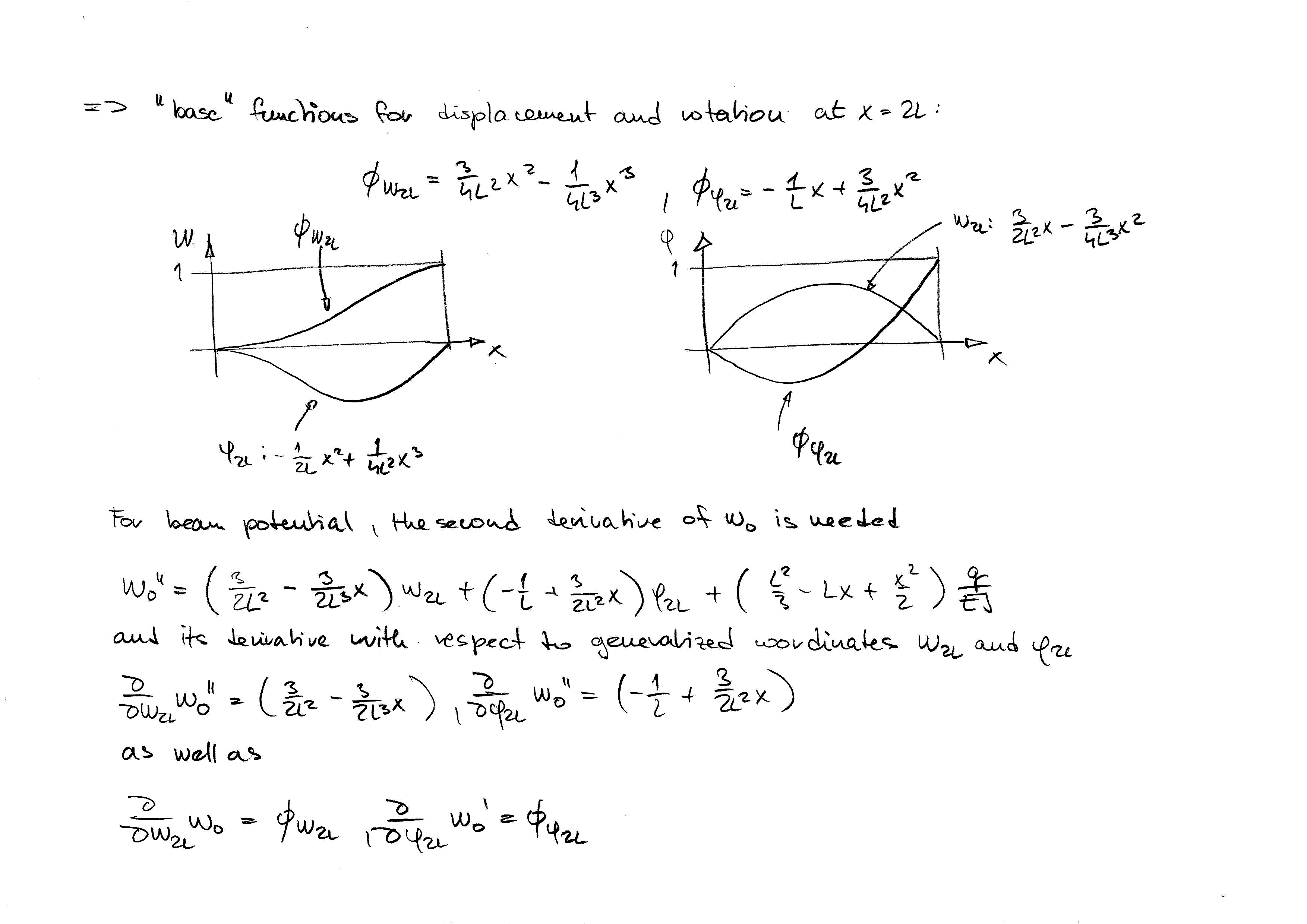
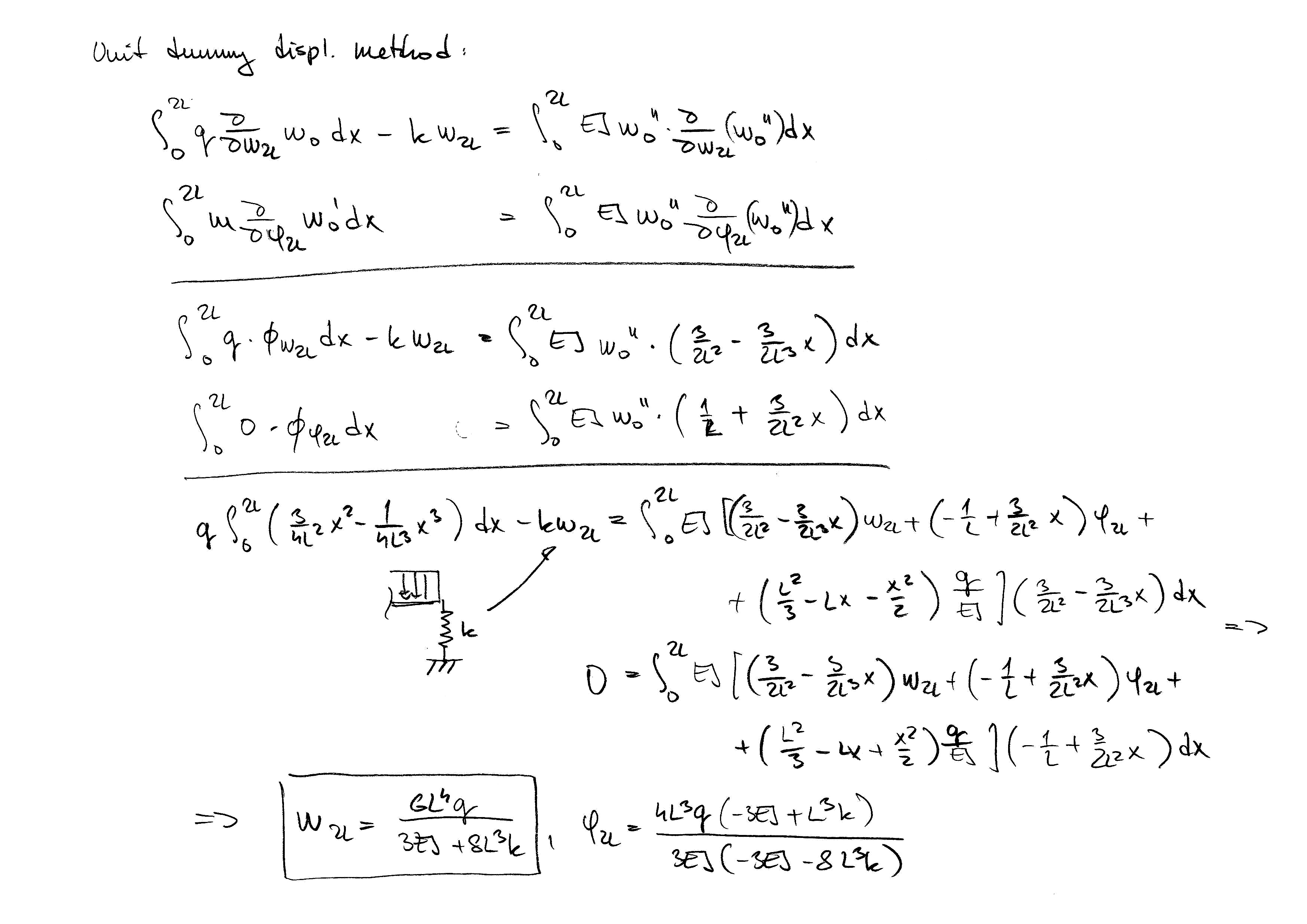
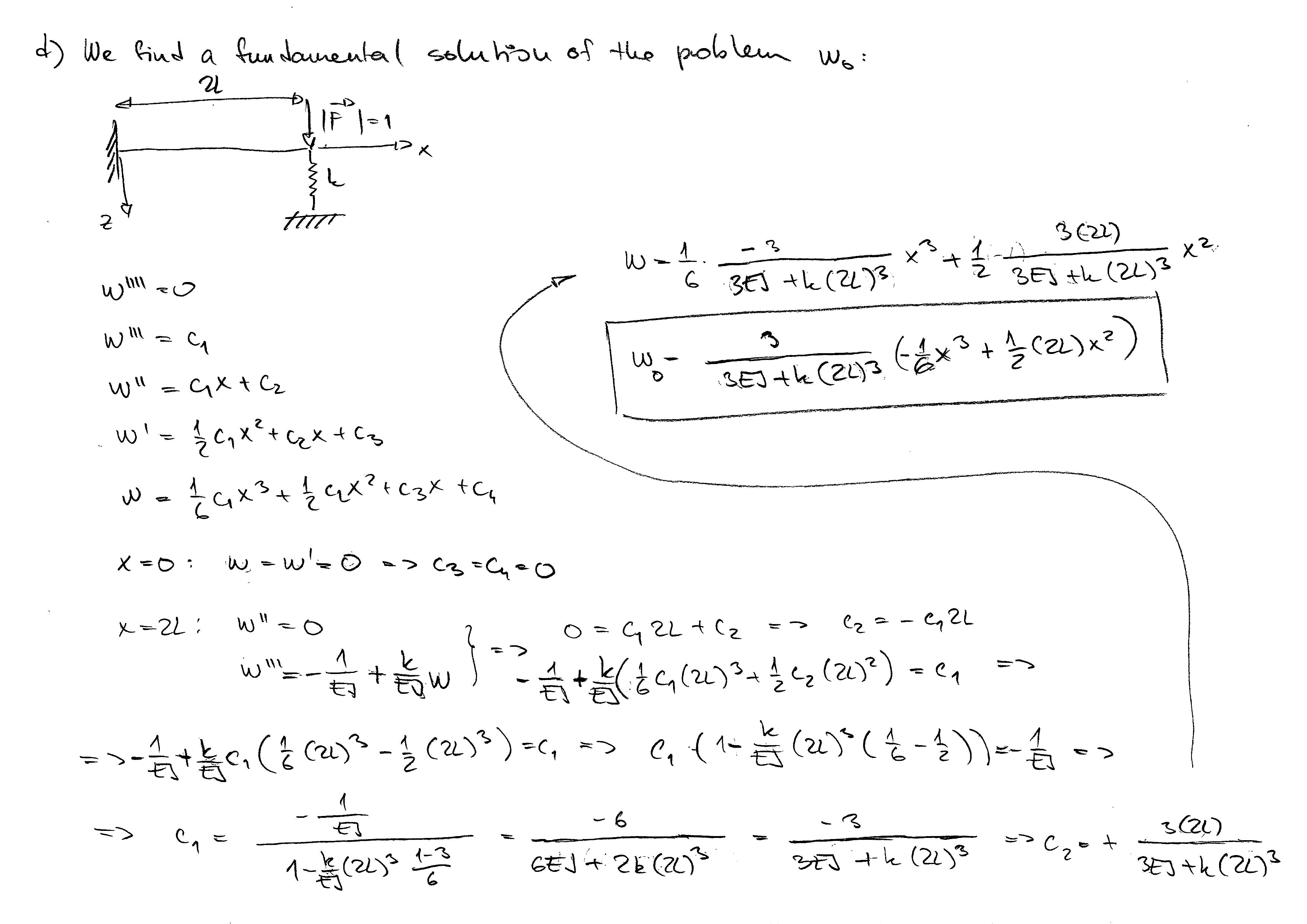
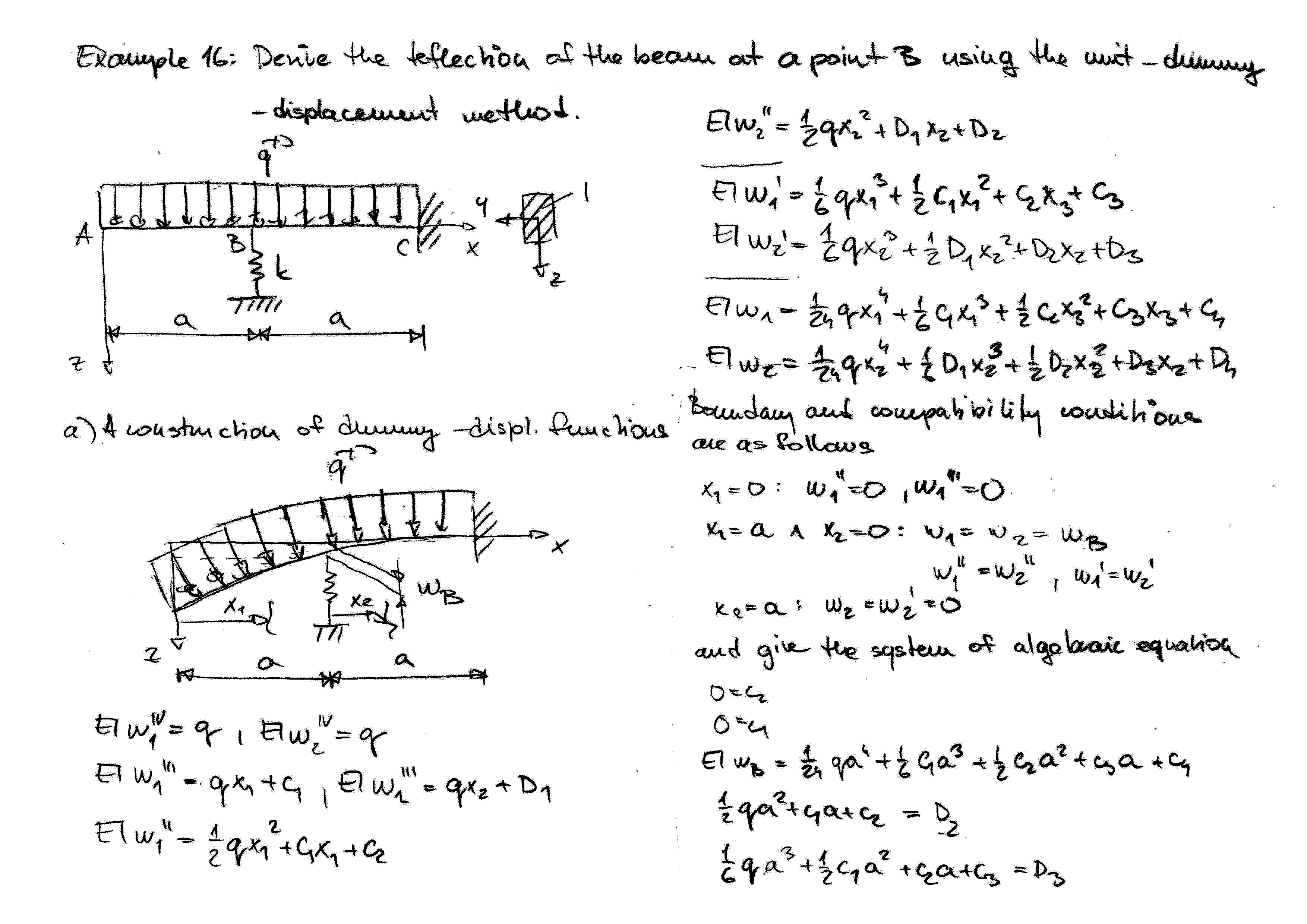
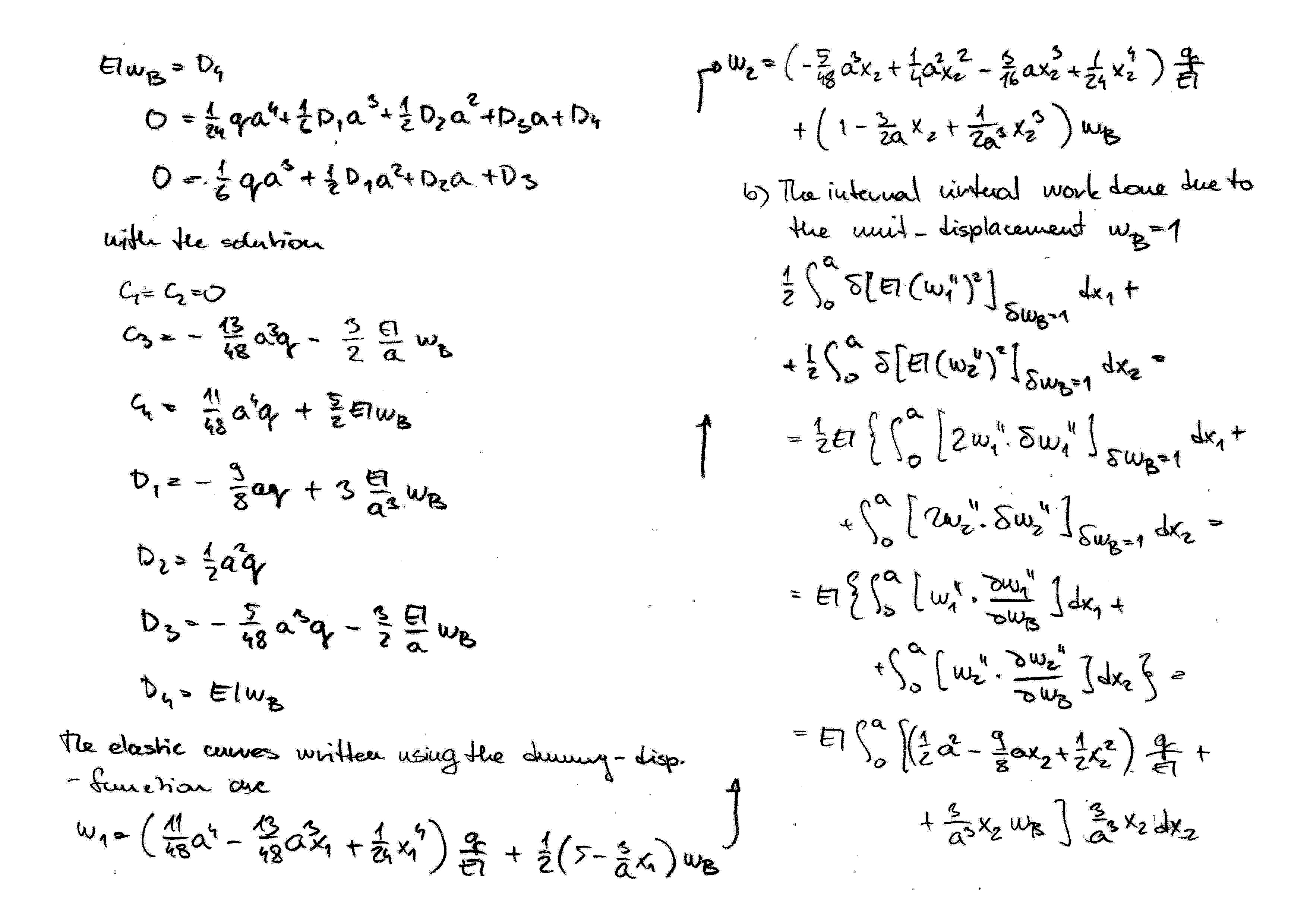
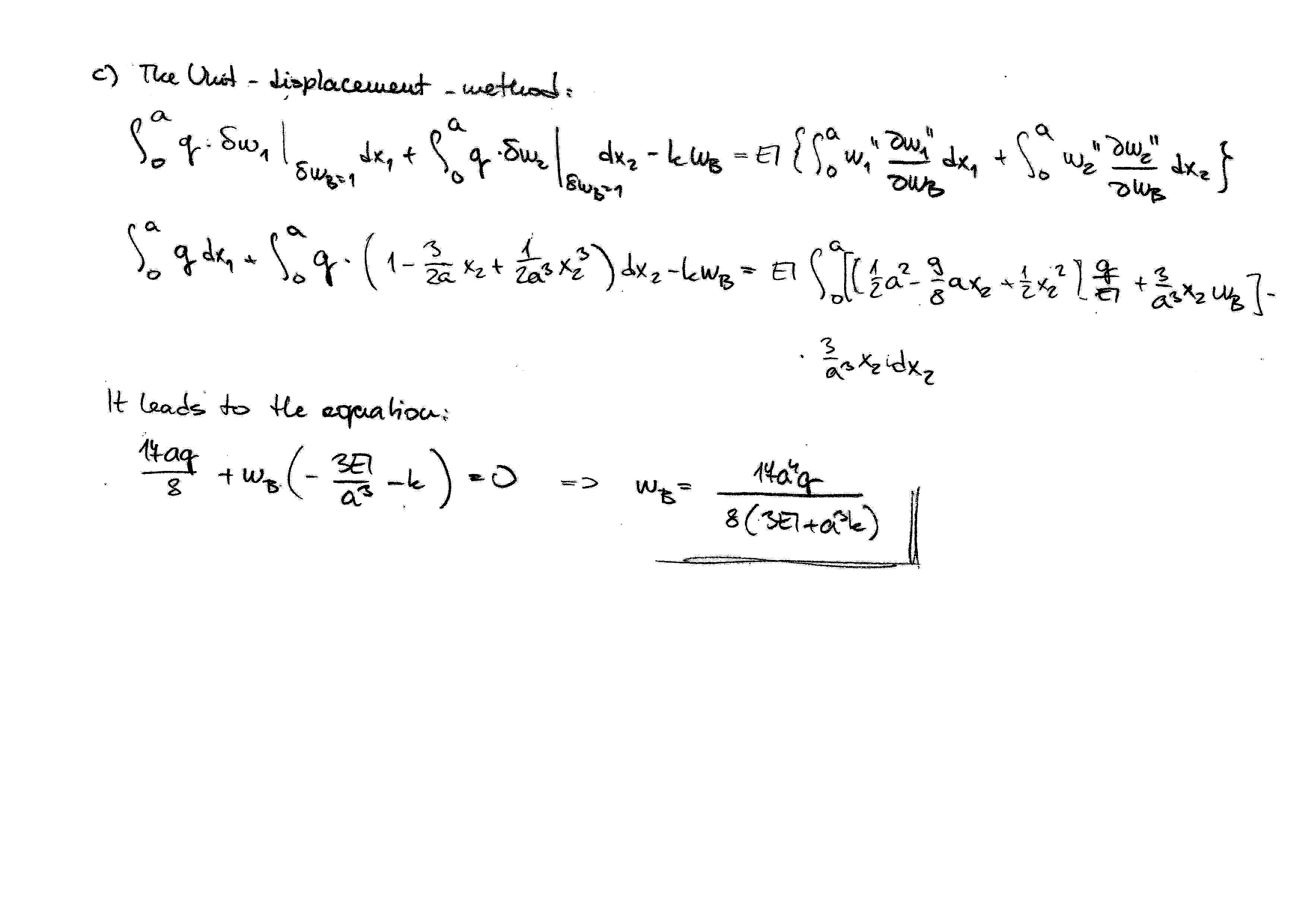
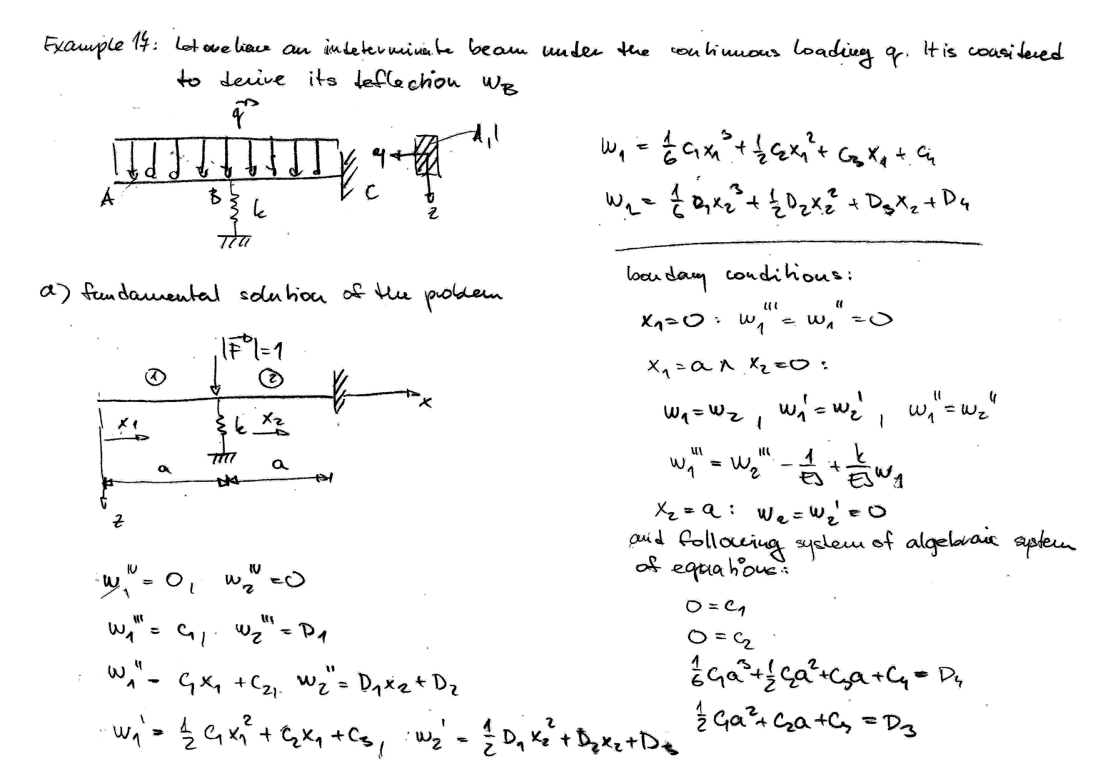
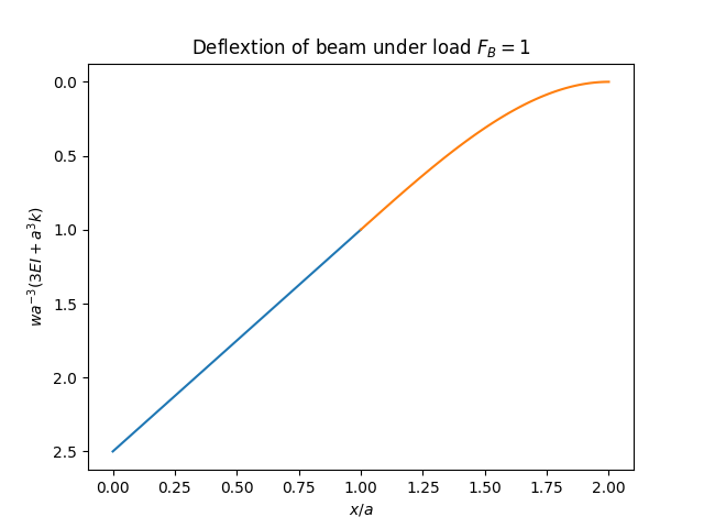
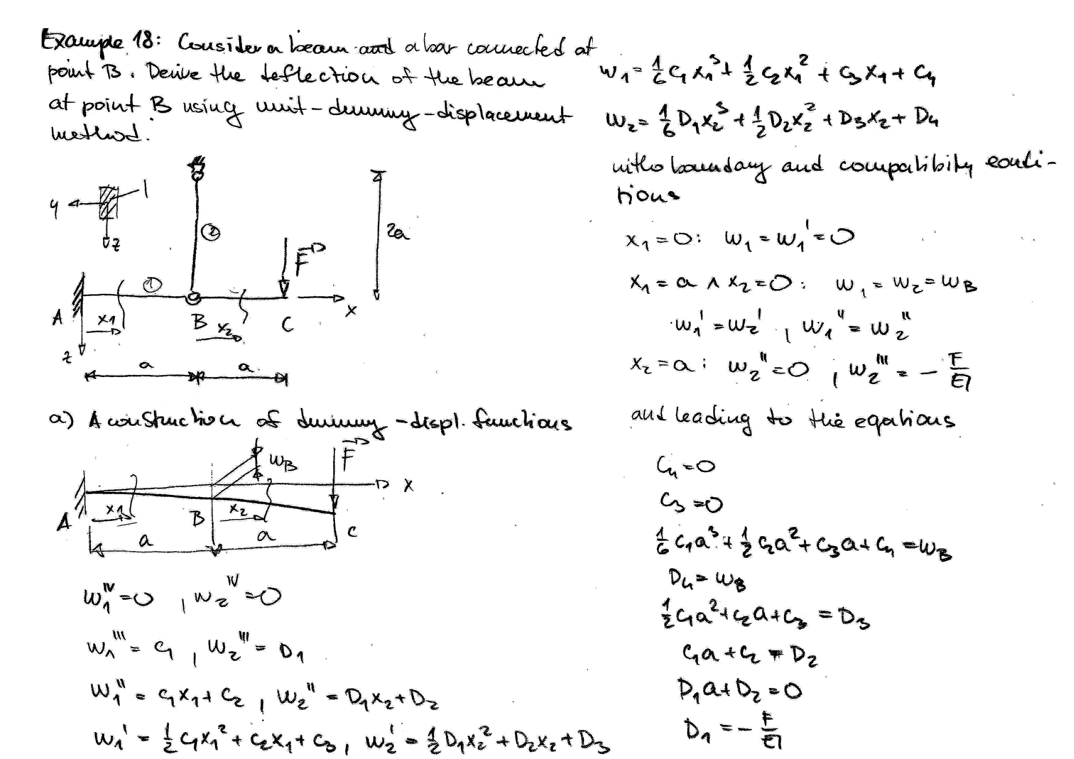
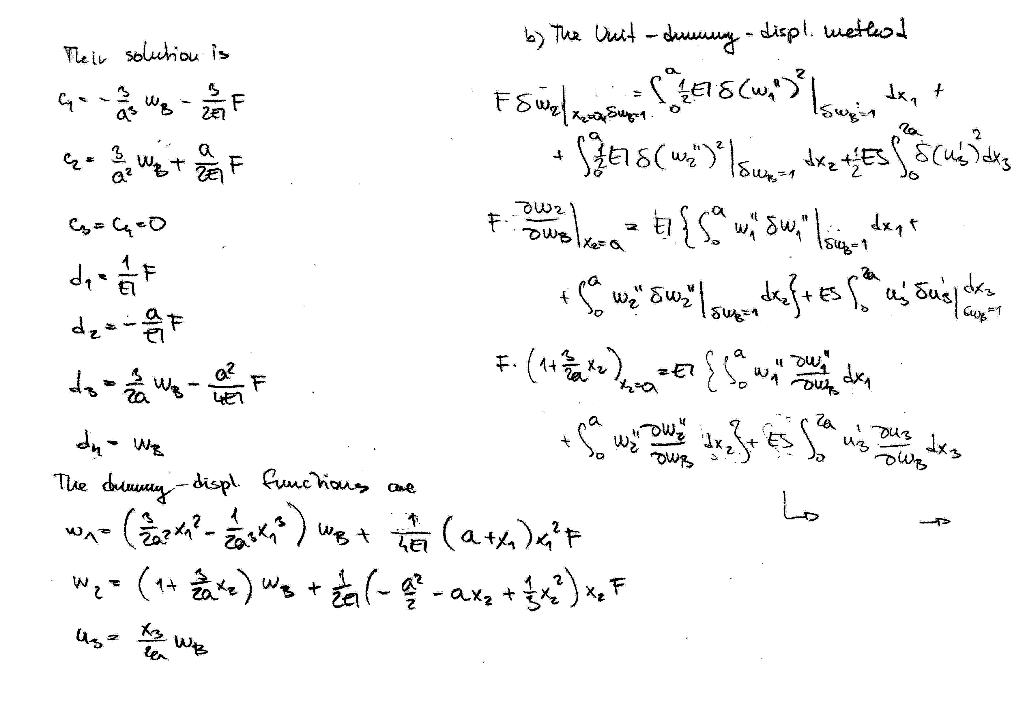
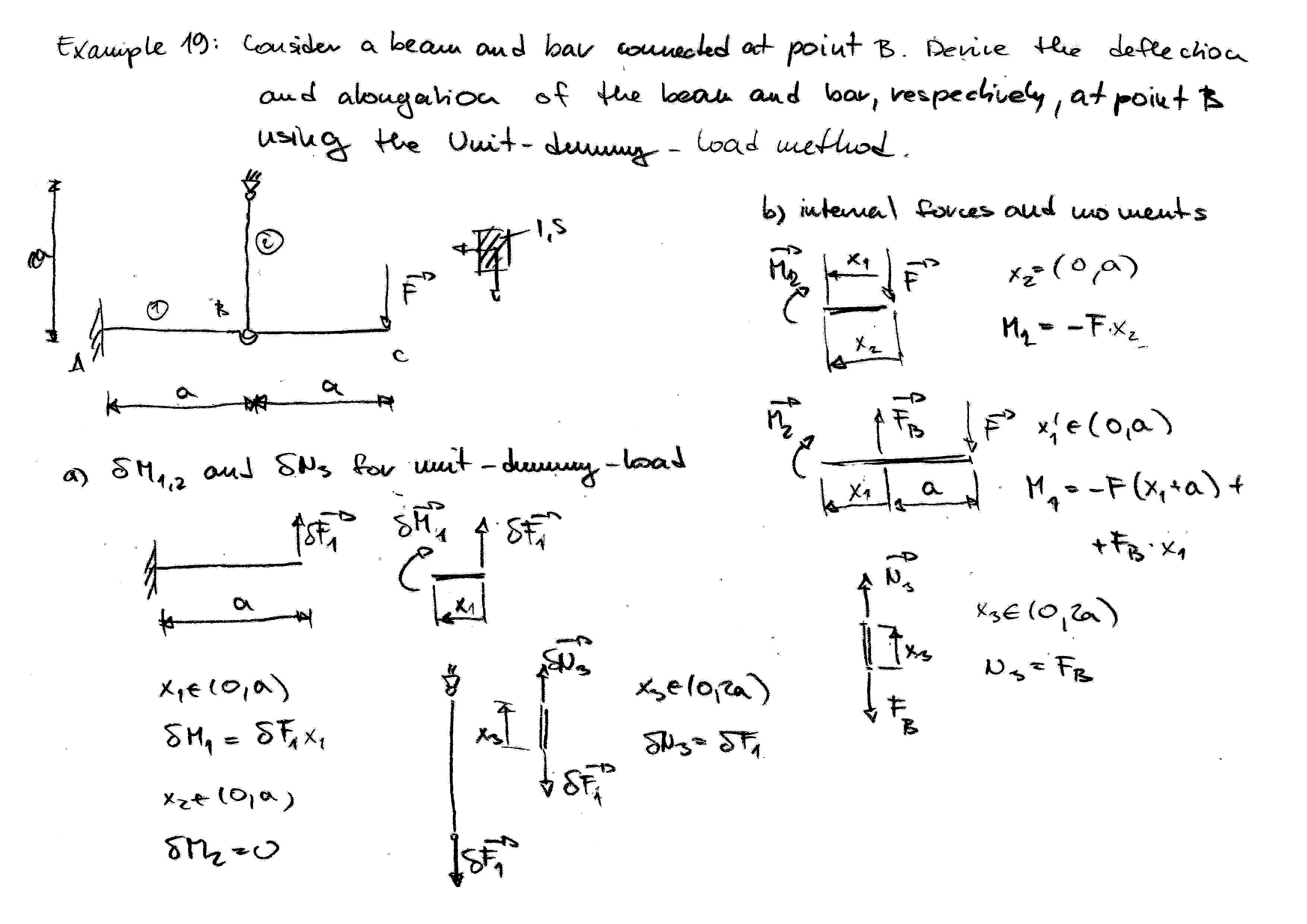
Unit-Dummy-Displacement Method
The principle of virtual work represented by equation (173) reduced to the form in the case of quasi-static loading process
can be used to directly determine reaction forces and displacements in structural problems. Consider the reaction force (or moment) \(\boldsymbol{R}_0\) at point \(0\) such, that
where \(\boldsymbol{e}_0\) is the unit vector in the direction of the reaction \(\boldsymbol{R}_0\). We prescribe a virtual displacement (or rotation) \(\delta\boldsymbol{u}_0\) as
at the point \(0\) in the elastic structure, but keep all other external forces on the structure stationary. The virtual strains \(\delta e_{ij}^0\) owing to the virtual displacement \(\delta u_0\) in the direction \(\boldsymbol{e}_0\) are determined from the kinematic considerations. Then the method of virtual work (183) reads as
or for \(\boldsymbol{f}=0\) as
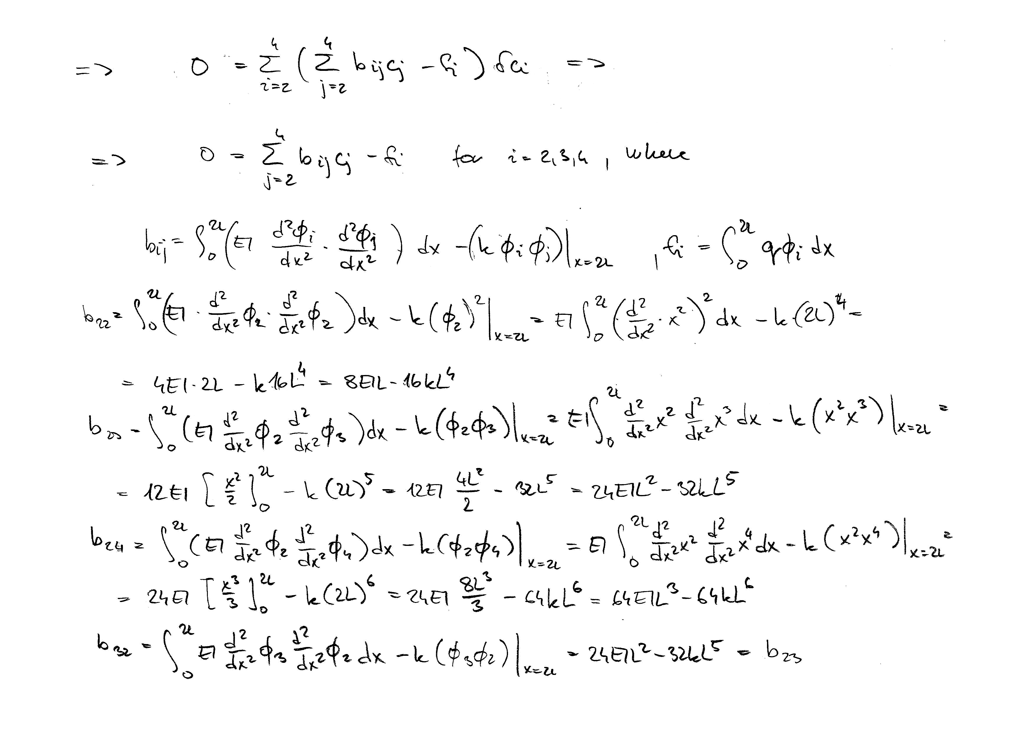
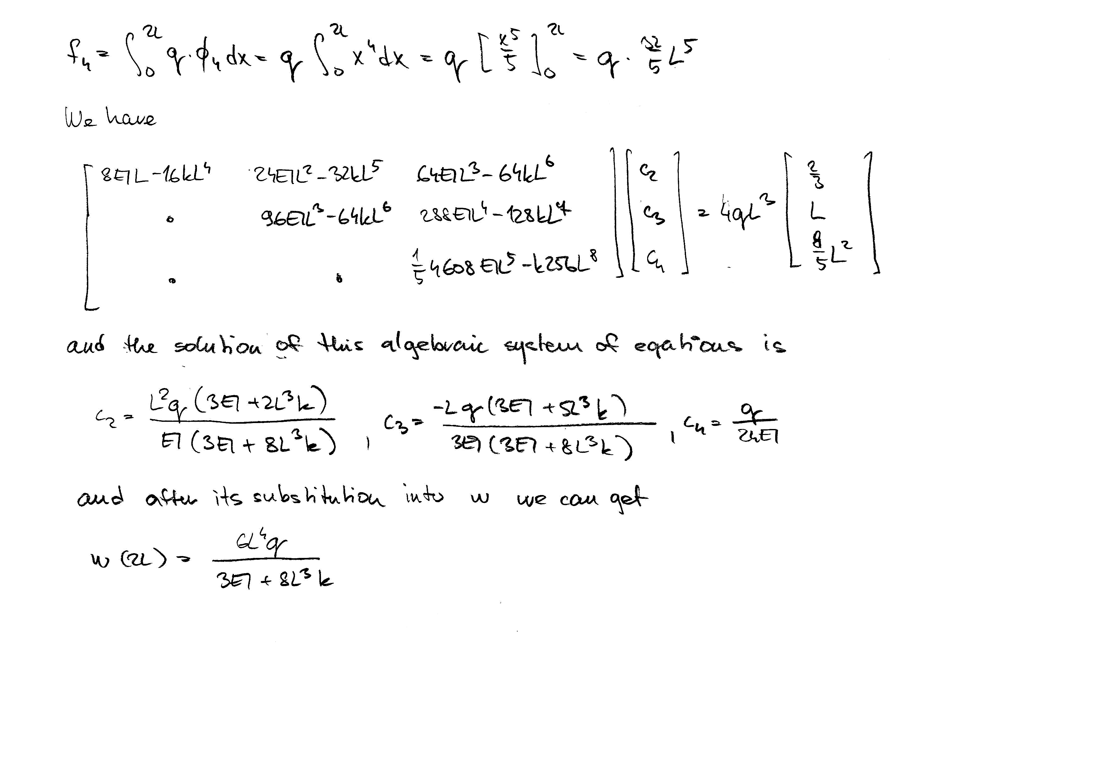
where \(\sigma_{ij}\) are the actual stresses and \(\delta e_{ij}^0\) or \(\delta u_i^0\) are the virtual strains or displacements, respectively, of the entire structure, consistent with the geometric constrains. Since \(\delta u_0\) is arbitrary, one can take \(\delta u_0=1\) and \(\delta e_{ij}^0\) or \(\delta u_i^0\) denote the virtual strains or displacements, respectively, corresponding to the unit displacement at point \(0\). This procedure is called the unit-dummy-displacement method and for the magnitude of the reaction \(\boldsymbol{R}_0\) we get
or if the volume loading \(\boldsymbol{f}\) is zero-valued
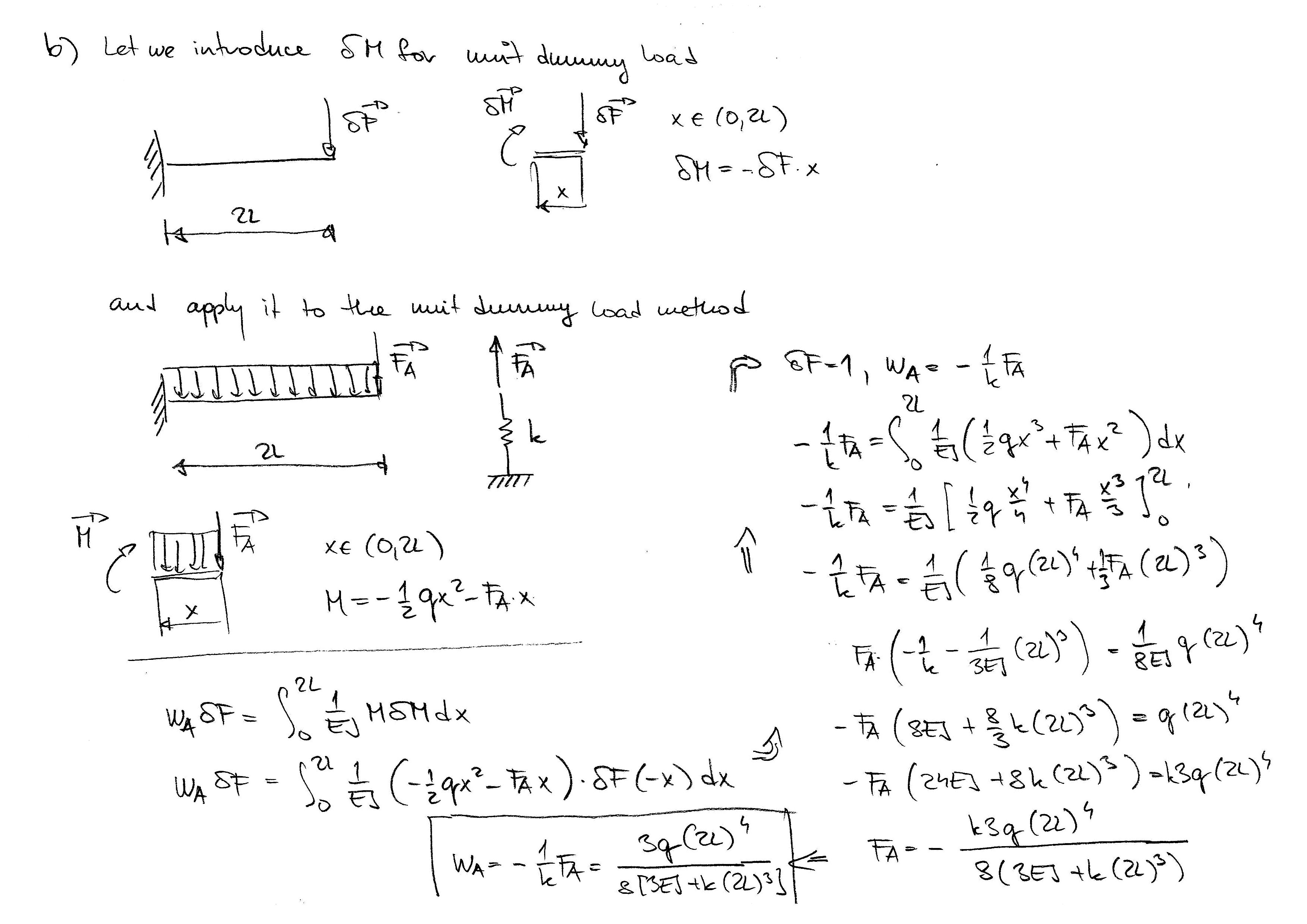
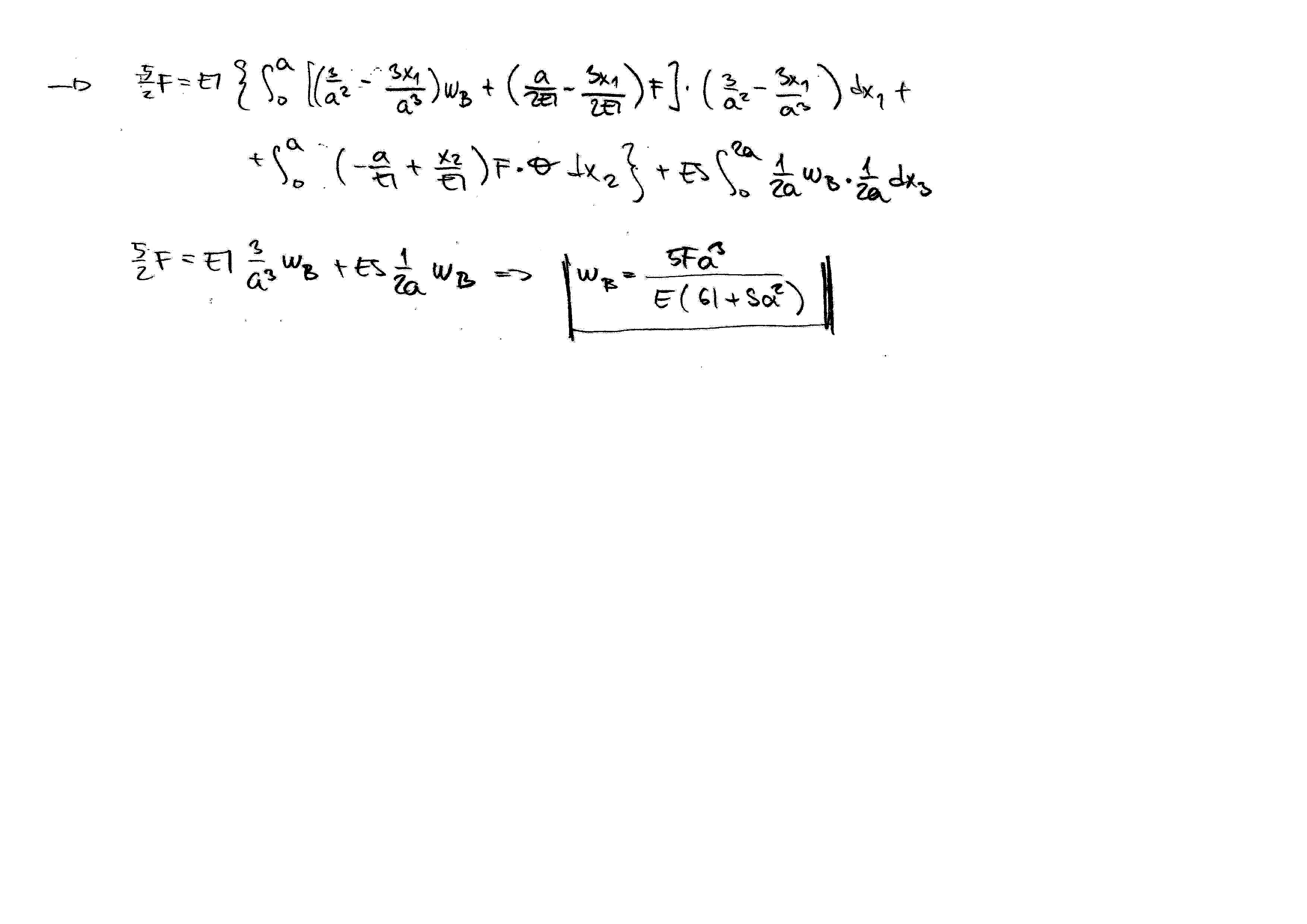
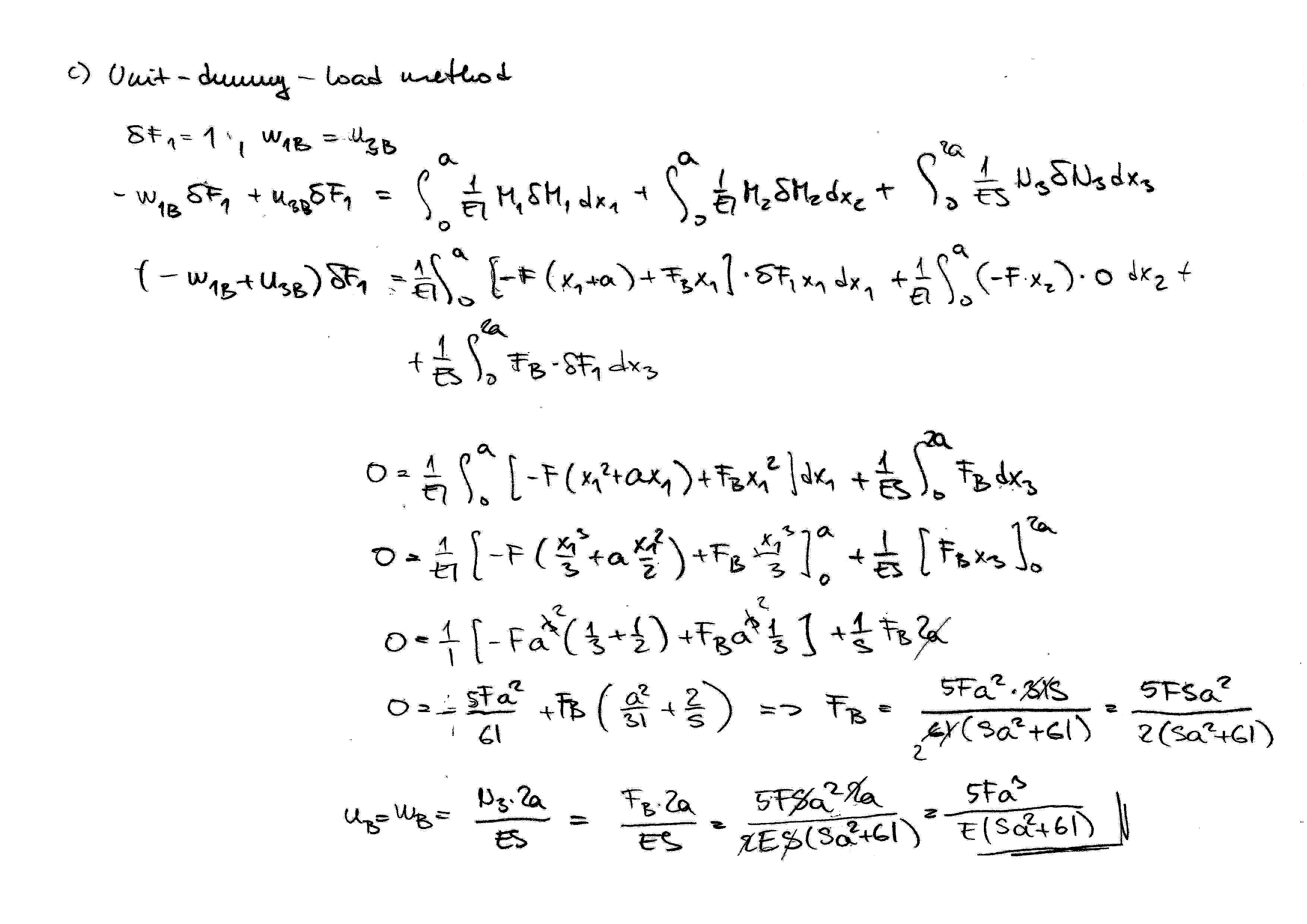
Unit-Dummy-Load Method
The basic idea can be described in analogy with the unit-dummy-displacement method. If the true displacement \(\boldsymbol{u}_0\) in the direction of the unit vector \(\boldsymbol{e}_0\), i.e.
is at the point \(0\) of an elastic structure, we can prescribe a virtual force \(\delta\boldsymbol{R}_0\) at that point and the same direction
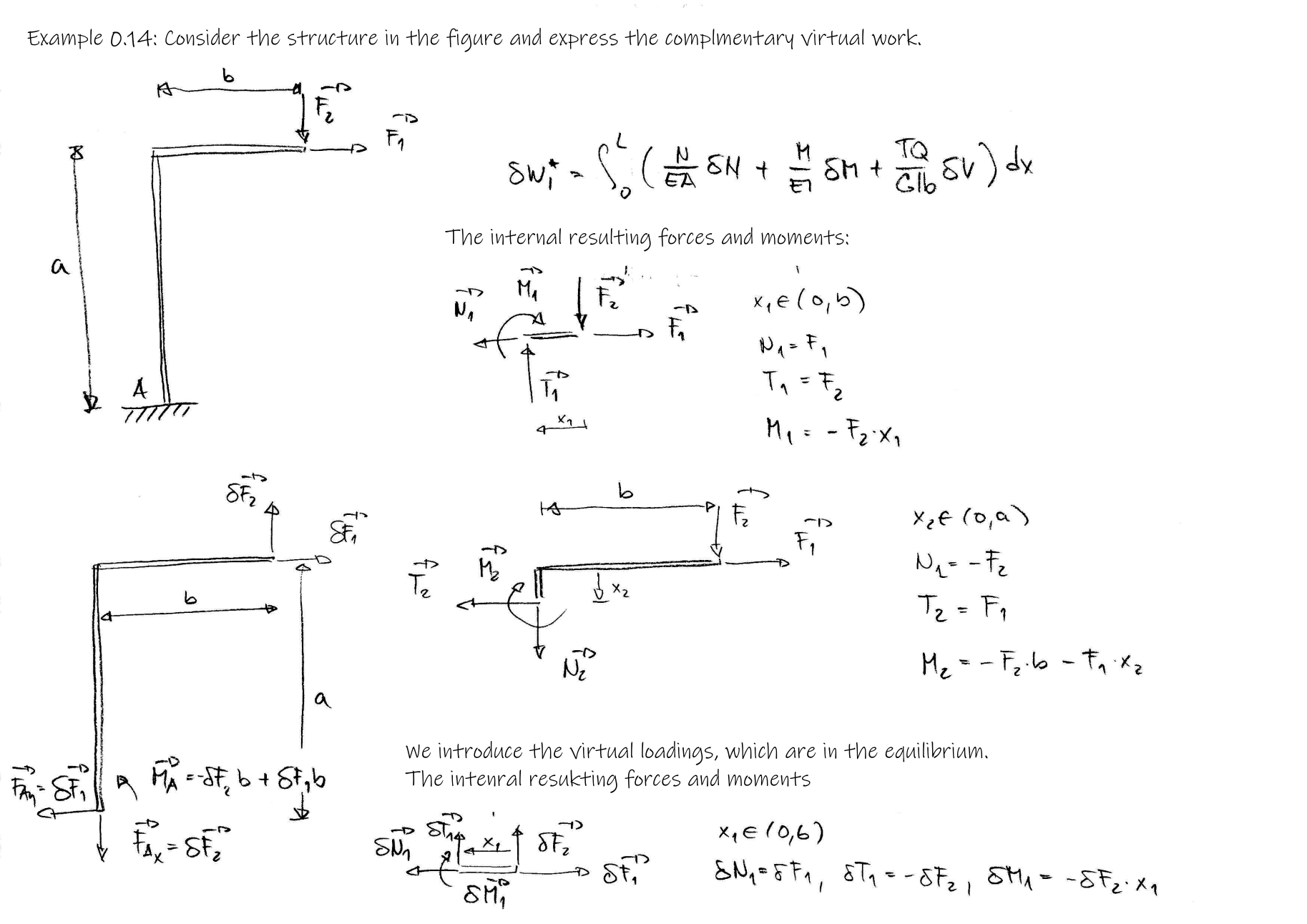
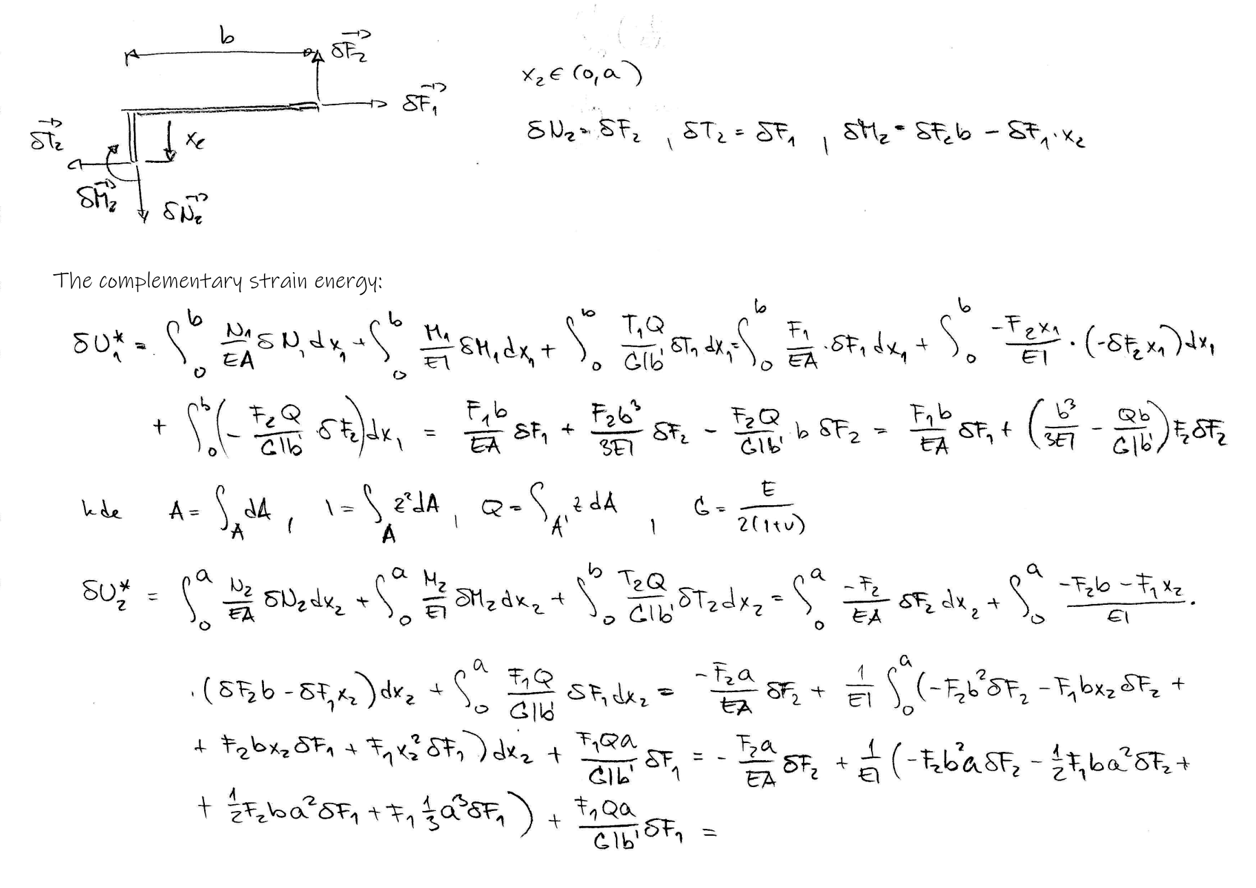
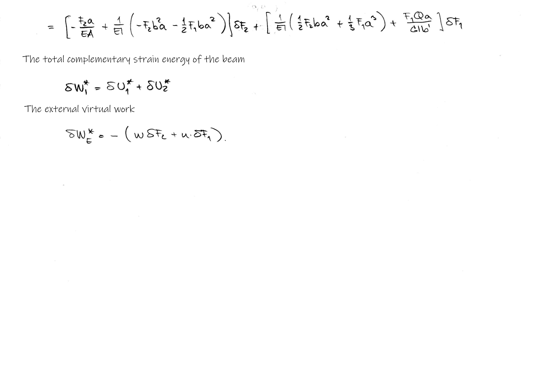
The application of virtual force induces a system of virtual stresses \(\delta\sigma_{ij}\) that satisfy the equilibrium equations. Then, instead of external work \(V\) and potential \(U\), their complementary counterparts \(V^*\) and \(U^*\) as the complementary potential energy \(\Pi^*\) is used in the Hamilton's principle. Then the principle of total complementary virtual work can be derive as follows
Consider
we have
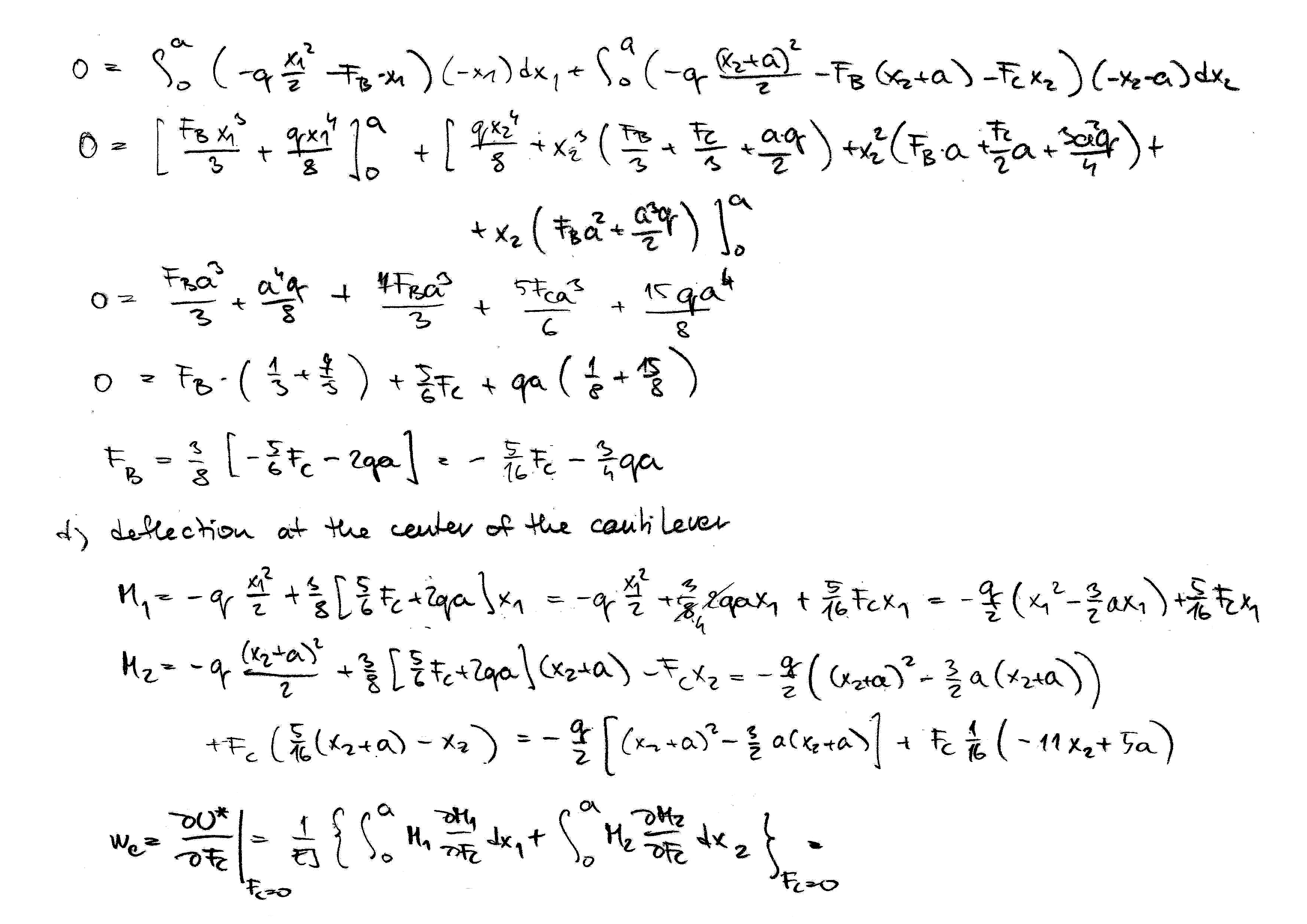
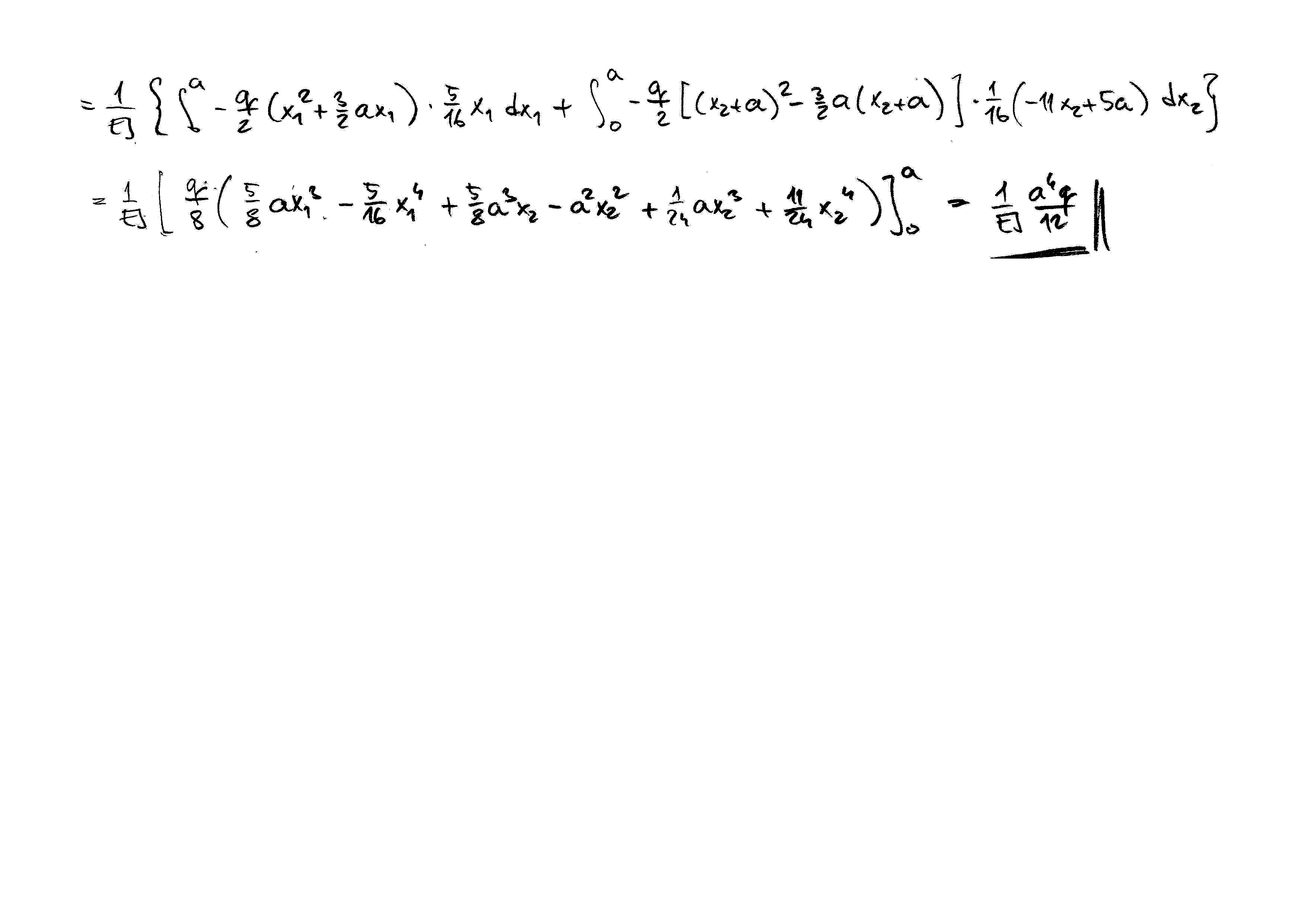
Once again we can take \(\delta R_0=1\) and calculate corresponding virtual internal stresses \(\delta\sigma_{ij}^0\) from equilibrium equations. From the previous equation consequently can be evaluated the magnitude of the true displacement \(\boldsymbol{u}_0\) as follows
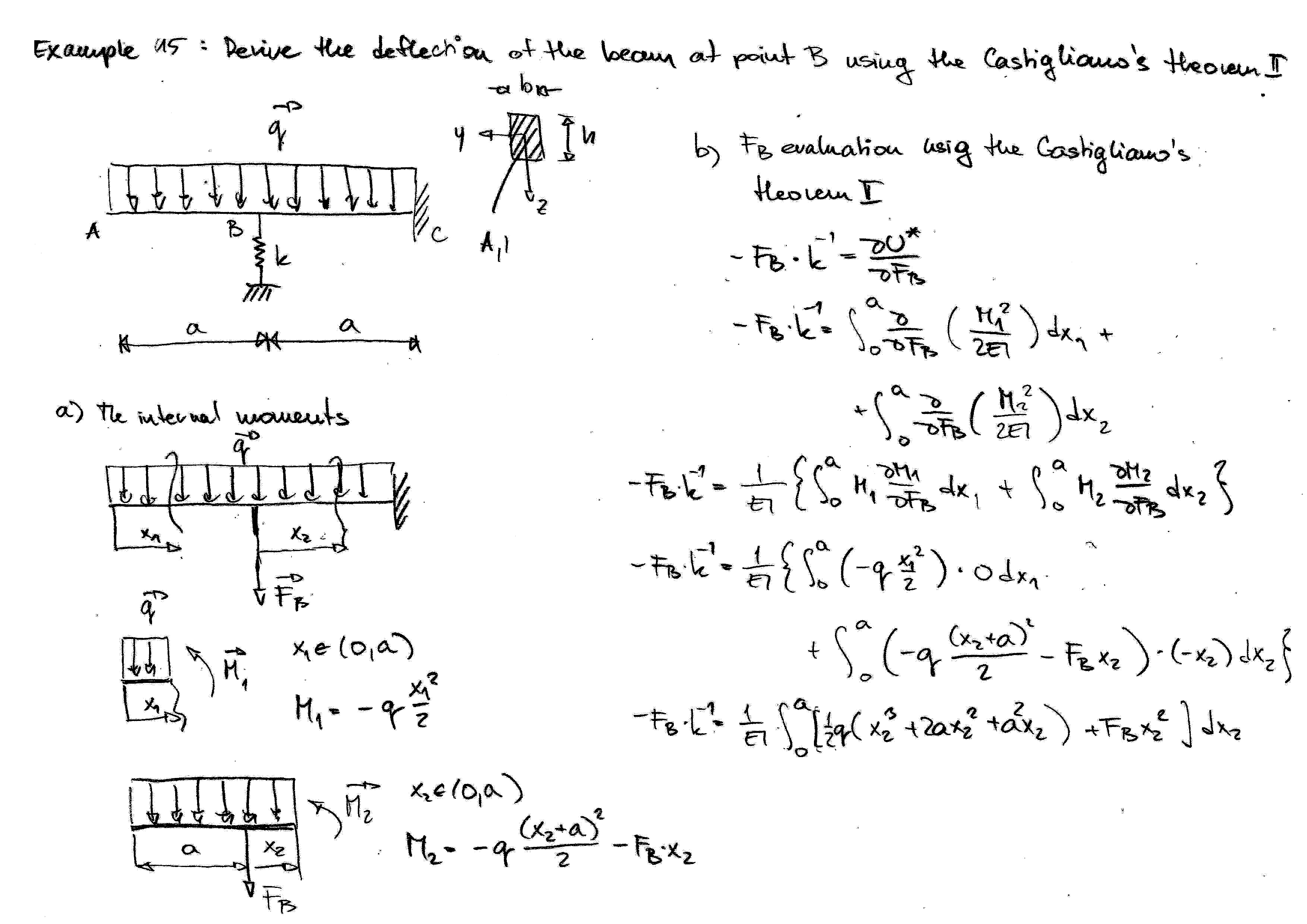
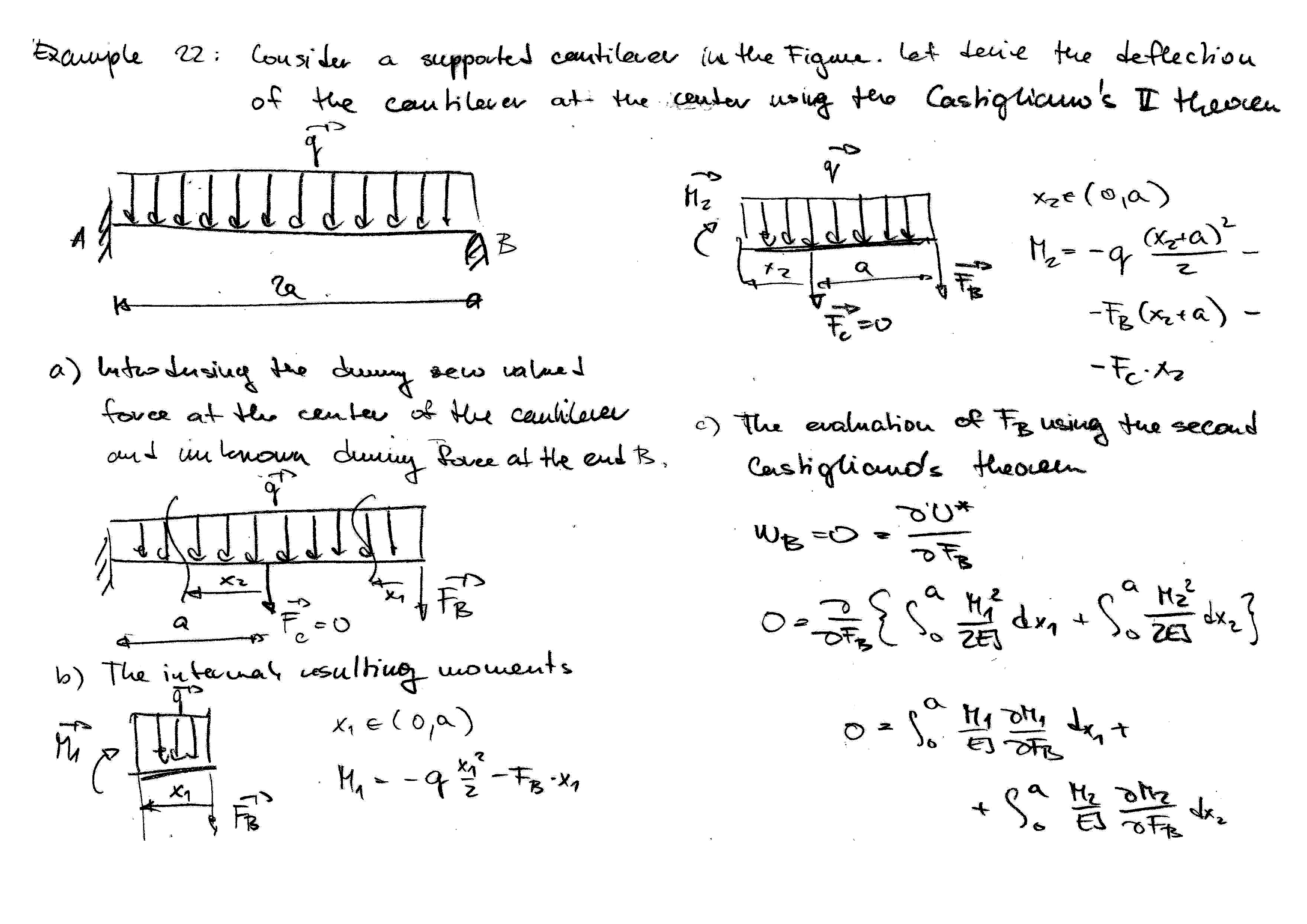
Castigliano's First Theorem
Consider a general three-dimensional structure that is in equilibrium under the action of \(N\) forces
where \(\boldsymbol{e}_i\) are unit vectors. Let
be the displacement corresponding to the forces \(\boldsymbol{F}_i\). The unit vector \(\boldsymbol{e}_i^\bot\) is orthogonal to the unit vector \(\boldsymbol{e}_i\) so the displacement component \(u_i^\bot\) does not contribute to the potential energy of the external forces \(V\), which is equal to
because the displacements \(u_i\) are points values, not functions of positions. It is also worth to note that the previous procedure can be used for moments \(\boldsymbol{M}_i\) and angles \(\boldsymbol{\theta}_i\). We assume that the displacement functions \(\boldsymbol{u}=\boldsymbol{u}(u_1,u_2,\dots,u_N)\) of the body can be expressed in terms of \(u_i\). Therefore, \(u_i\) serve as the generalized coordinates and the strain energy \(U\) of the body can be expressed in terms of \(u_i\), \(i=1,2,\dots,N\). The total potential energy of the body is given by
For any virtual variation \(\delta u_i\) in the displacement \(u_i\), the variation \(\delta\Pi\) in the total potential energy \(\Pi\) must vanish
Since the variations \(\delta u_1,\delta u_2,\dots,\delta u_N\) are independent of each other, it follows that
or for \(\boldsymbol{f}=0\) the simplified expression is obtained
Equation (201) is the general statement of Castigliano's first theorem: If the strain energy of a structural system can be expressed in terms of \(N\) independent displacements \(u_1,u_2,\dots,u_N\) corresponding to \(N\) specified forces \(F_1,F_2,\dots,F_N\), the first partial derivative of the strain energy with respect to any displacement \(u_i\) (under the load \(F_i\)) is equal to the force \(F_i\) in the direction of \(u_i\).
The first Castigliano's theorem is a special case of the principle of virtual displacements and equivalent to the unit-dummy-displacement method if the virtual strains and displacements of the entire structure \(\delta e_{ij}^0\) and \(\delta u_i^0\) for unit displacement \(\delta u_0=1\) in (188) are differentiable with respect to \(u_0\) and can be written to the form
Then substituting these relations into (188) leads to
which is equation (201) for \(i=0\).
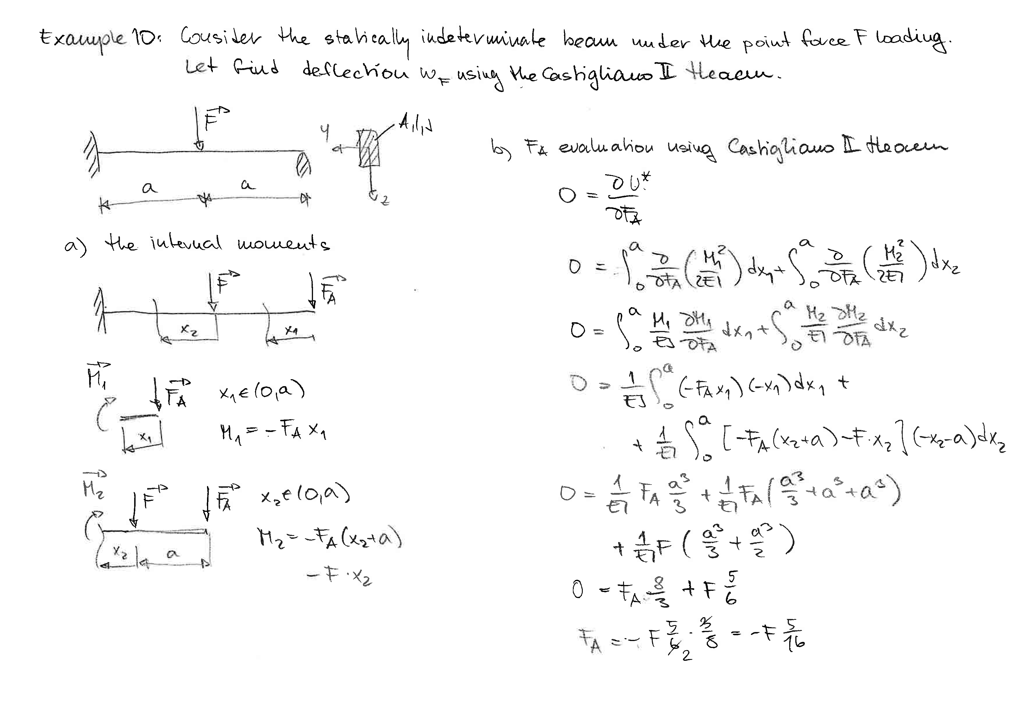
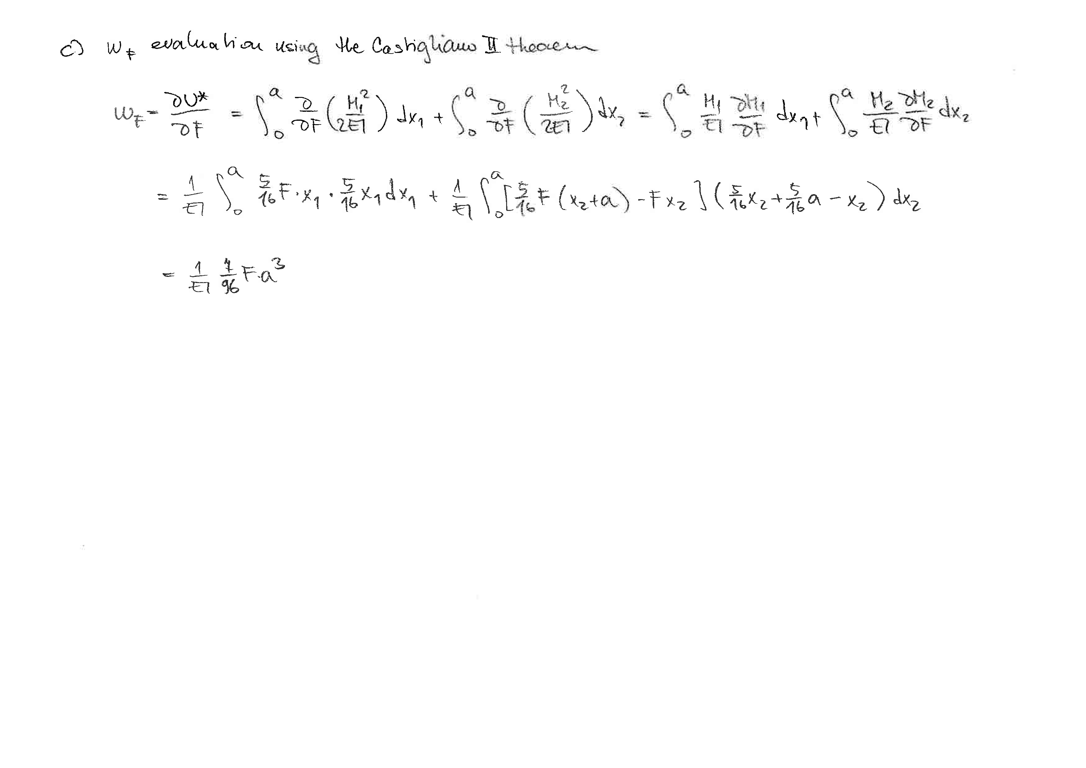
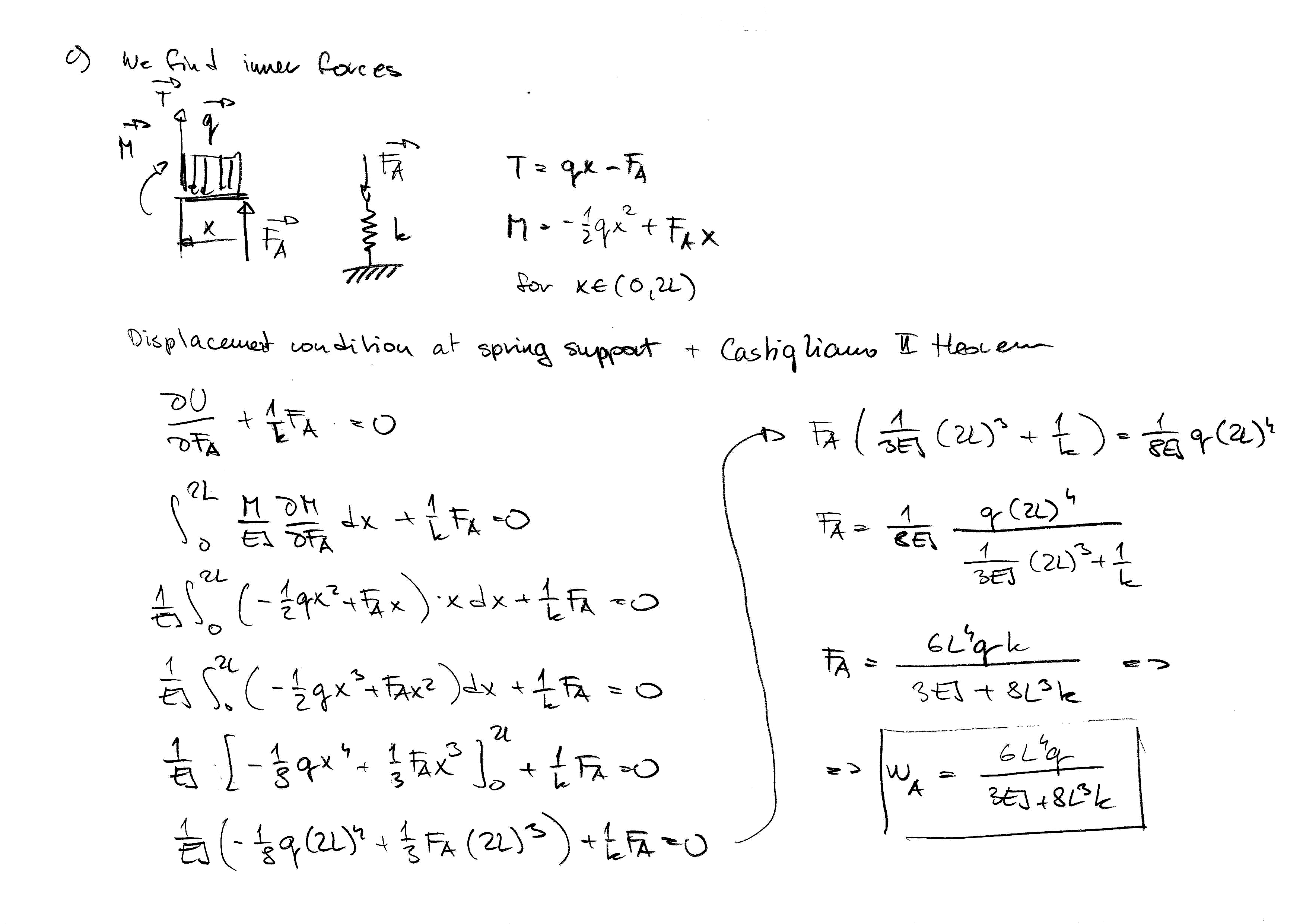
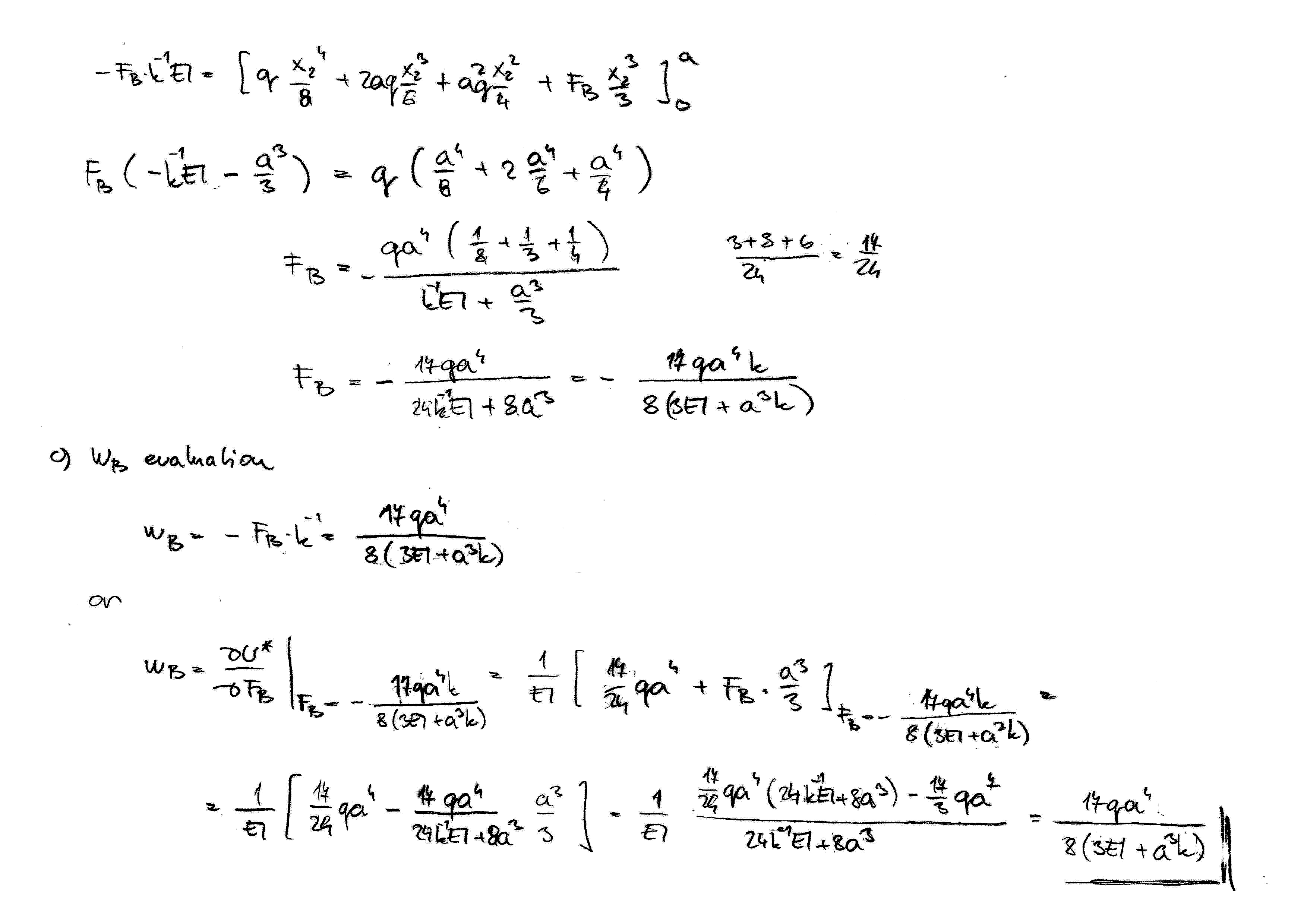
Castigliano's Second Theorem
Contrary to the first Castigliano's theorem, the second one is based on the total complementary energy principle. If a structural system is in equilibrium under the action of \(N\) forces
where \(\boldsymbol{e}_i\) are unit vectors, then the same procedure as presented for the first Castigliano's theorem leads for the complementary energy \(U^*=U^*(F_1,F_2,\dots,F_N)\) to the equation
This equation represents the Castigliano's second theorem and \(u_i\) is the component of the displacement \(\boldsymbol{u}_i\) at the point of the point force \(\boldsymbol{F}_i\), which is in the direction of the unit vector \(\boldsymbol{e}_i\). Equation (206) is valid for structures that are linearly elastic as well as nonlinearly elastic. When they are linearly elastic, we have \(U=U^*\) and one can express the strain energy in terms of displacements \(U=U(u_i)\) or forces \(U=U(F_i)\). Hence, the unit-dummy-load method is equivalent to the Castigliano's second theorem.
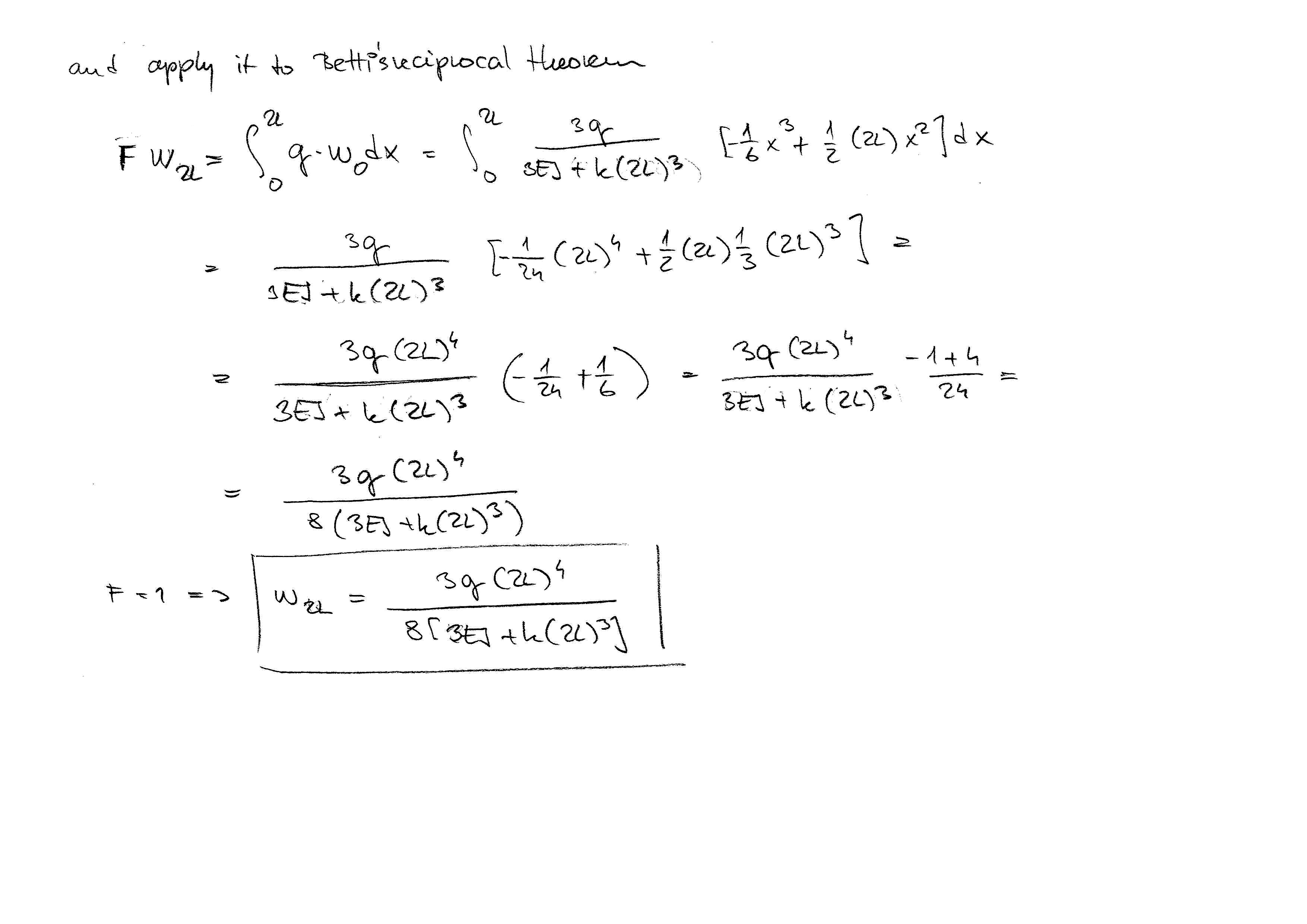
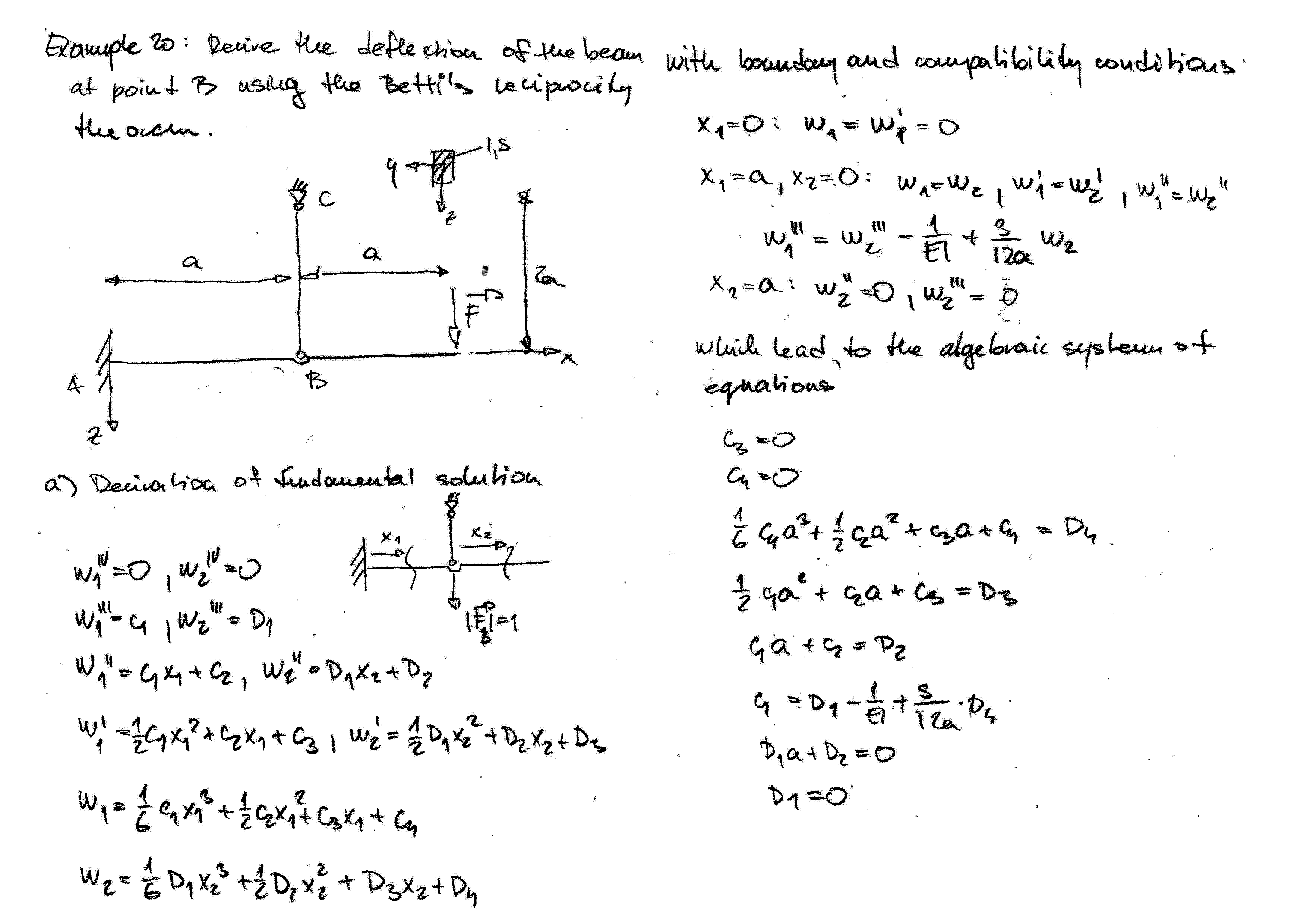
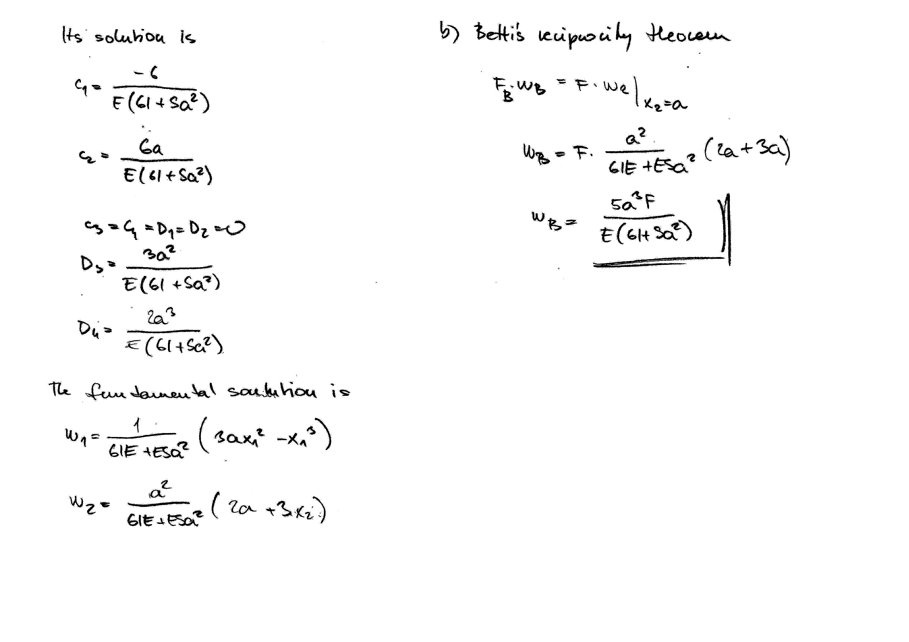
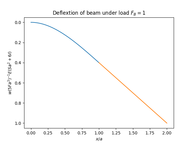
Betti's and Maxwell's Reciprocity Theorems
The principle of superposition is said to be hold for a linear elastic body if the displacements obtained under a given set of forces is equal to the sum of the individual displacements that would be obtained by applying the single forces separately. On the other hand, the principle of superposition is not valid for strain and potential energies, because they are quadratic functions of displacements or forces. In other words, when a linear elastic body is subjected to more than one external force, the total work caused by external forces is not equal to the sum of the works that are obtained by applying the single forces separately.
Consider a linear elastic solid that is in equilibrium under the action of two external forces \(F_1\) and \(F_2\). Since the order of application of the forces is arbitrary, we suppose that force \(F_1\) is applied first. Let \(W_1\) be the work produced by \(F_1\). Then, we apply force \(F_2\), which produces work \(W_2\). This work is the same as that produced by force \(F_2\), if it alone were acting on the body. When force \(F_2\) is applied, force \(F_1\), which is already acting on the body, does additional work, because its point of application is displaced, owing to the deformation caused by force \(F_2\). Let us denote this work by \(W_{12}\). Thus the total work done by the application of forces \(F_1\) and \(F_2\) is
Work \(W_{12}\), which can be positive or negative, is zero if and only if the displacement of the point of application of force \(F_1\) produced by force \(F_2\) is zero or is perpendicular to the direction of \(F_1\). Now we change the order of application. Then the total work done is equal to
where \(W_{21}\) is the work done by force \(F_2\), because of the application of force \(F_1\). The work done in both cases should be the same because, at the end, the elastic body is loaded by the same pair of external forces. Thus we have
Equation (209) is a mathematical statement of the Betti's reciprocity theorem. Applied to a three-dimensional elastic body, (209) takes the form
where \(\overline{u}_i\) are the displacements produced by the body forces \(\overline{f}_i\) and surface forces \(\overline{t}_i\), and \(u_i\) are the displacements produced by body forces \(f_i\) and surface forces \(t_i\). Hence, the Betti's reciprocity theorem states: if a linear elastic body is subjected to two different set of forces, the work done by the first system of forces in moving through the displacements produced by the second system of forces is equal to the work done by the second system of forces in moving through the displacements produced by the first system of forces.
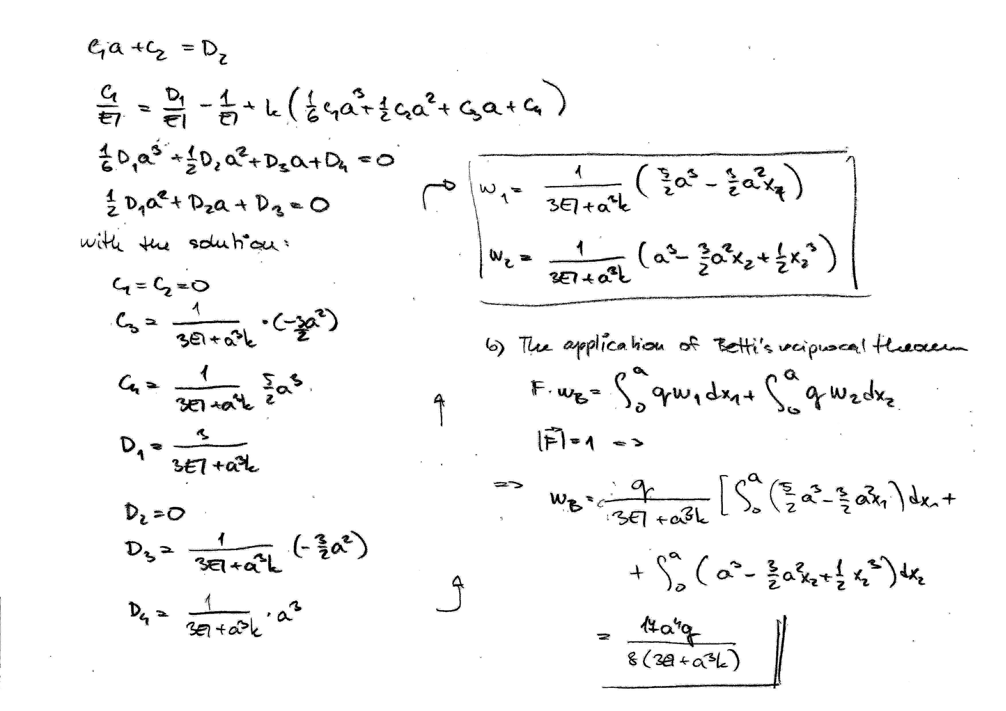
Consider a linear elastic solid subjected to force \(\boldsymbol{F}_A\) of unit magnitude acting at point \(A\) and force \(\boldsymbol{F}_B\) of unit magnitude acting at a different point \(B\) of the body. Let \(\boldsymbol{u}_{AB}\) be the displacement of point \(A\) in the direction of force \(\boldsymbol{F}_A\) produced by unit force \(\boldsymbol{F}_B\), and \(\boldsymbol{u}_{BA}\) be the displacement of point \(B\) in the direction of force \(\boldsymbol{F}_B\) produced by unit force \(\boldsymbol{F}_A\). From Betti's theorem it follows that
or
It is a statement of Maxwell's theorem, which states: if the displacement \(u_{AB}\) of point \(A\) in the direction of unit force \(\boldsymbol{F}_A\) produced by unit force \(\boldsymbol{F}_B\) acting at point \(B\) is equal to the displacement \(u_{BA}\) of point \(B\) in the direction of unit force \(\boldsymbol{F}_B\) produced by a unit force \(\boldsymbol{F}_A\) acting at point \(A\).
Downloads 9:
Lecture 9 to download
hereas the pdf presentation.Example 9.3 to download
here,here,here,here,here,here,hereahere.Example 9.5 to download
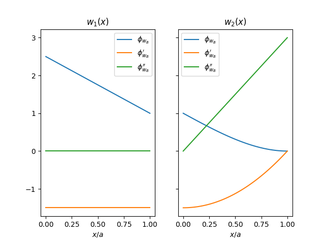
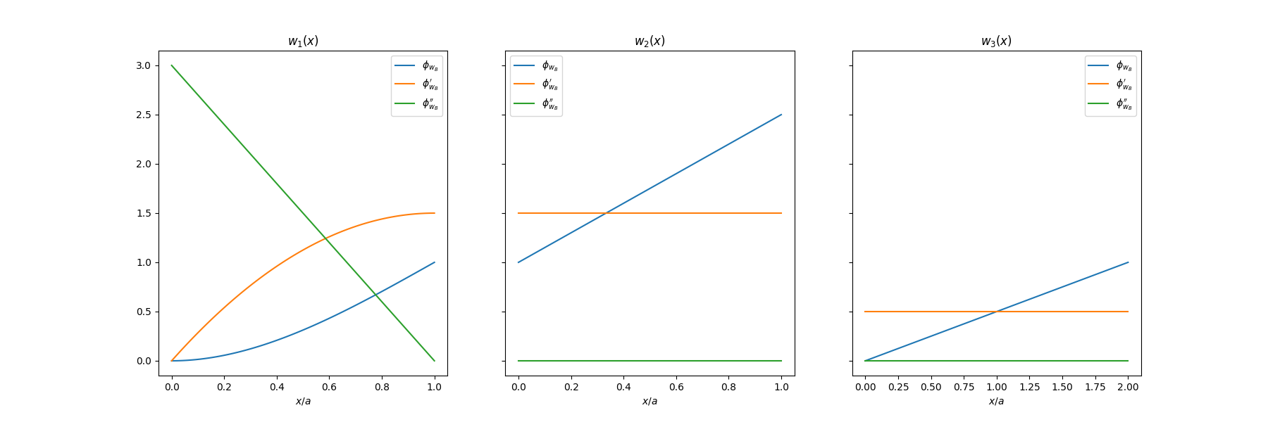
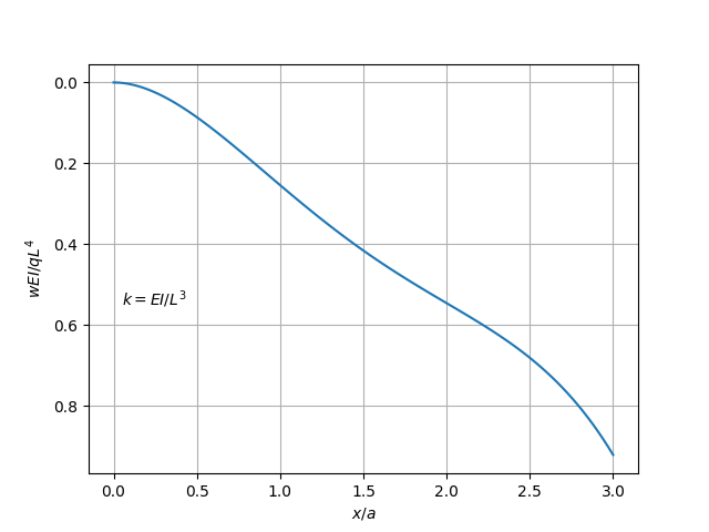
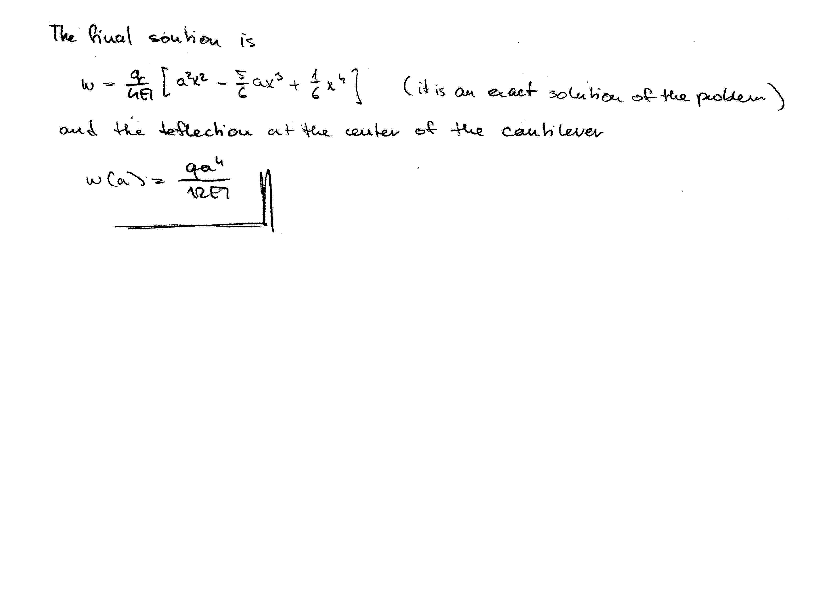
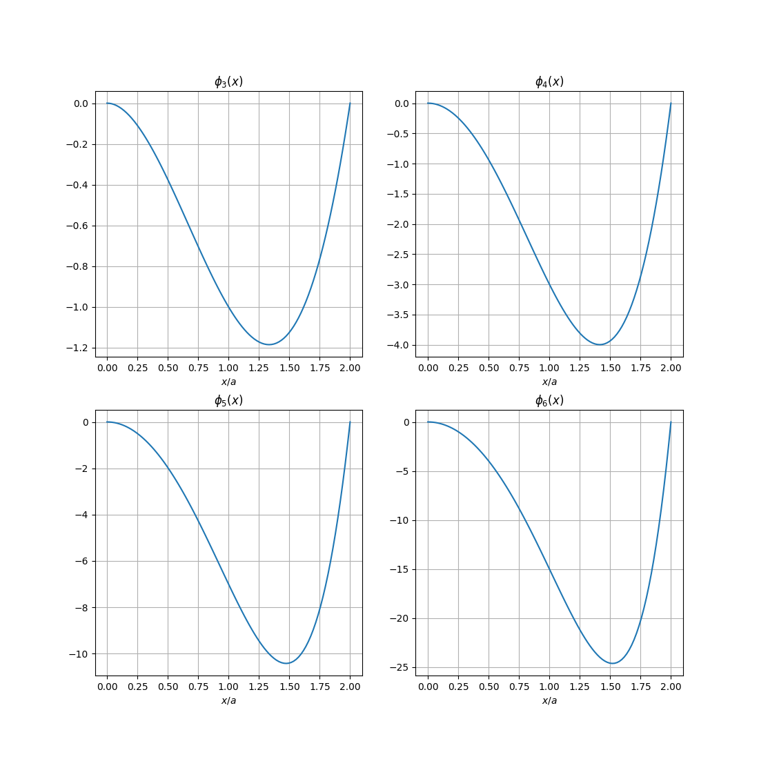
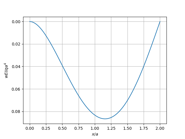
here,hereandhere. The auxiliary script in Python finding the solution of the system of algebraic equations and dummy functions can be downloadedhere. The graphs of the displacement dummy functions arehere.Example 9.6 to download
hereandhere. The auxiliary script in Python finding the solution of the system of algebraic equations and fundamental solution can be downloadedhere. The graph of the fundamental solution ishere.Example 9.7 to download
here,hereandhere. The auxiliary script in Python finding the solution of the system of algebraic equations and dummy functions can be downloadedhere. The graph of dummy functions arehere.Example 9.9 to download
hereandhere. The auxiliary script in Python finding the solution of the system of algebraic equations and fundamental solution can be downloadedhere. The graph of the fundamental solution ishere.
Lecture 10
In the principle of virtual displacements, the Euler equations are the equilibrium equations, whereas in the principle of virtual forces, they are the compatibility equations. The Euler equations are in the form of differential equations that are not always tractable by exact methods of solution. The direct variational methods usually bypass the derivation of the Euler equations and go directly from a variational statement of the problem to the solution of the Euler equations. One of these methods is the Ritz method and the Galerkin method.
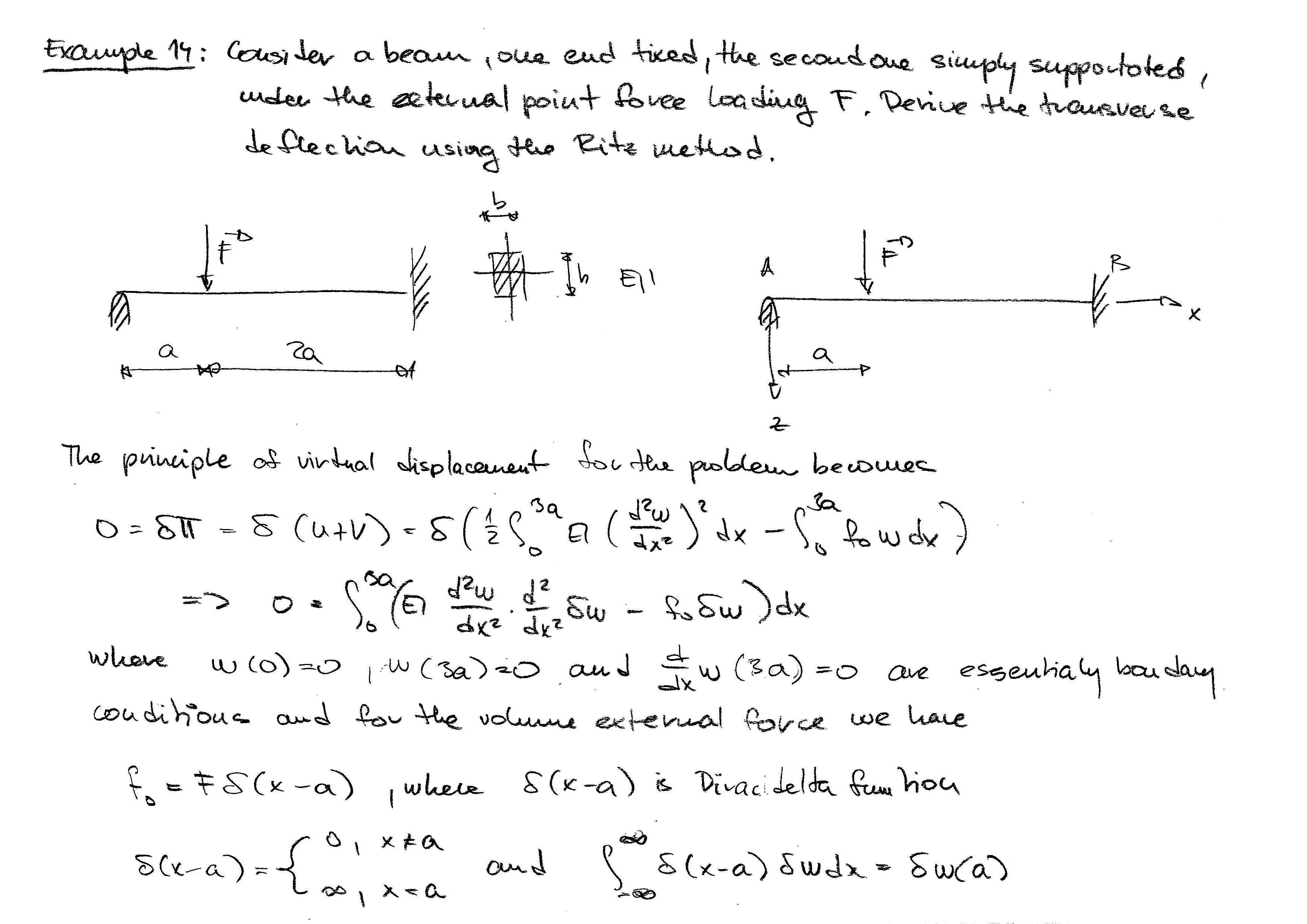
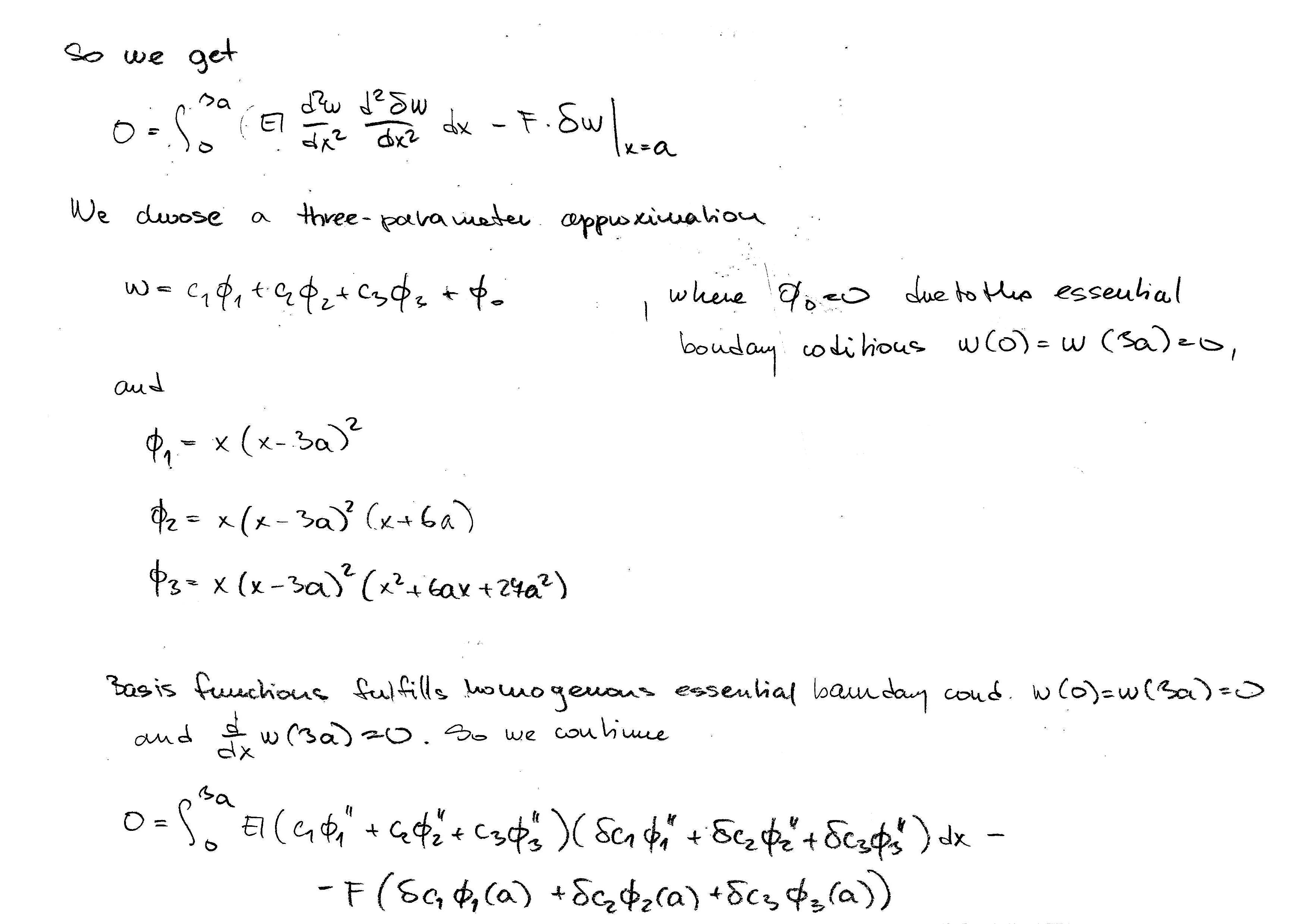
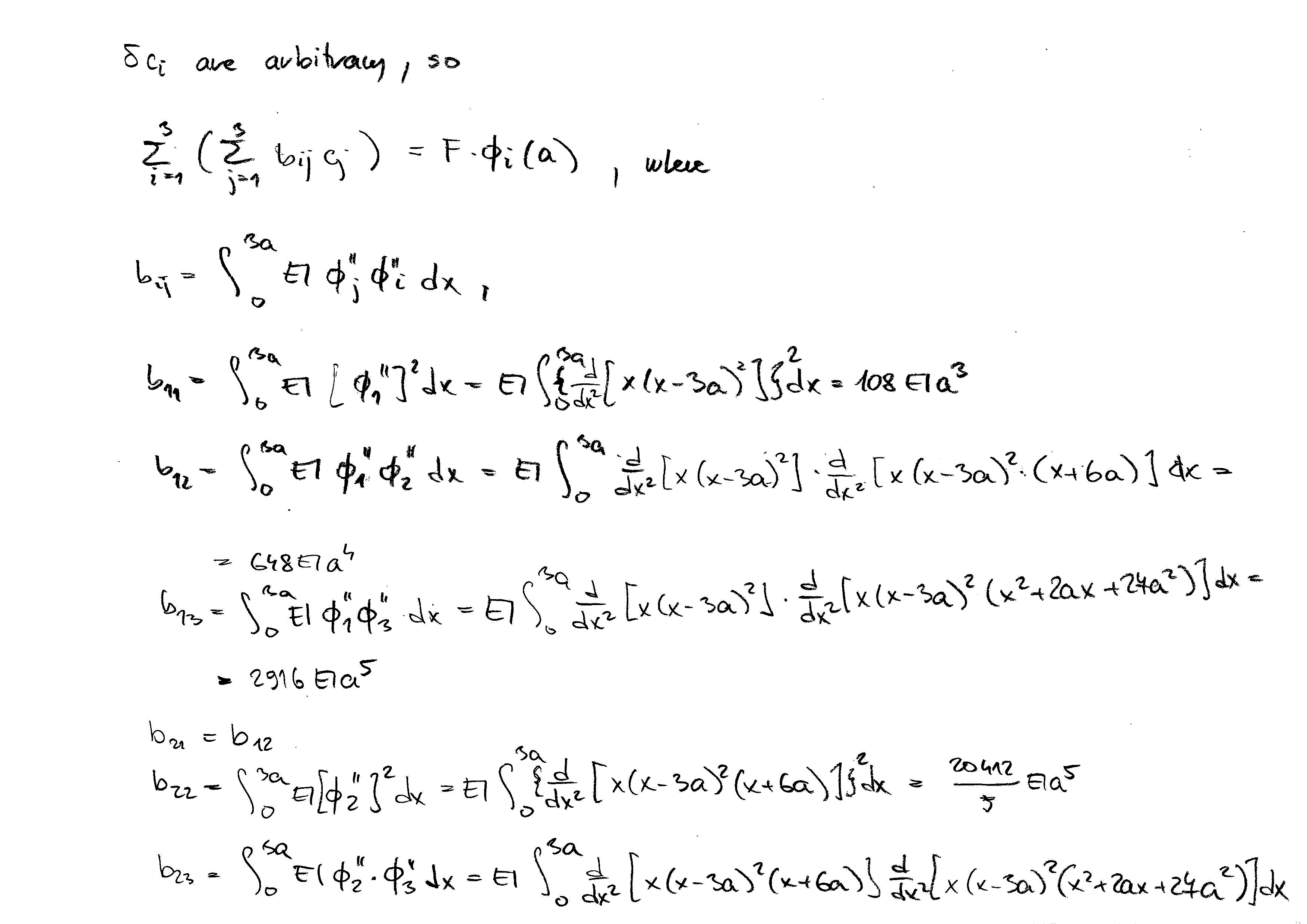
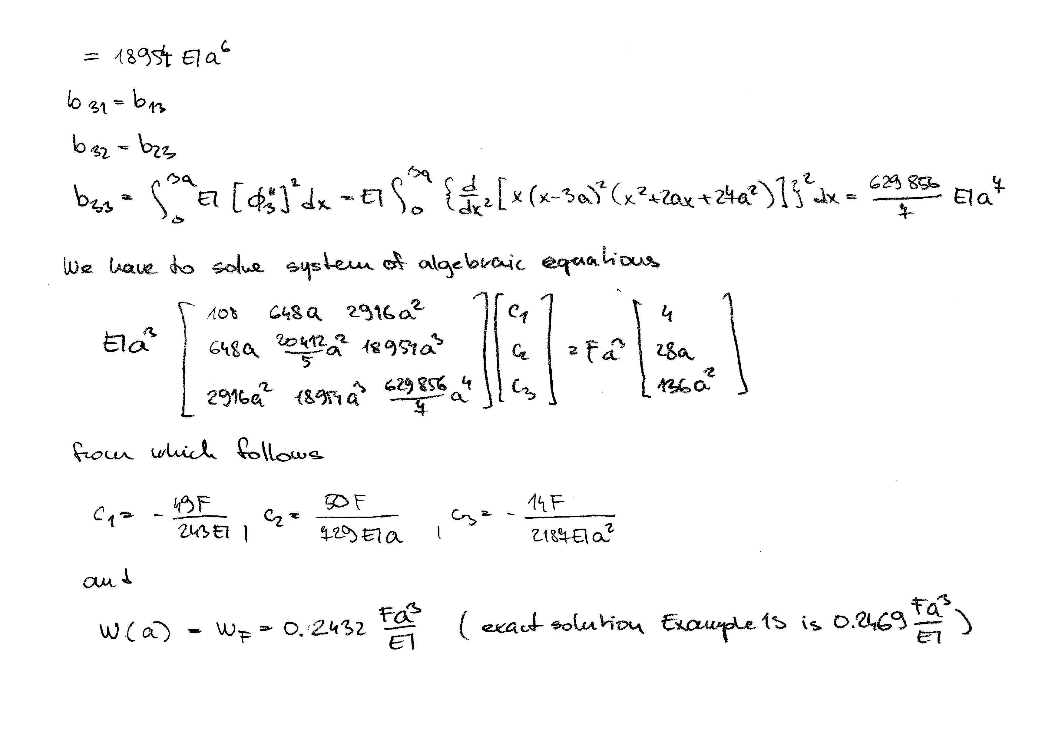
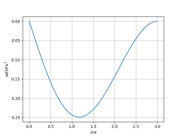
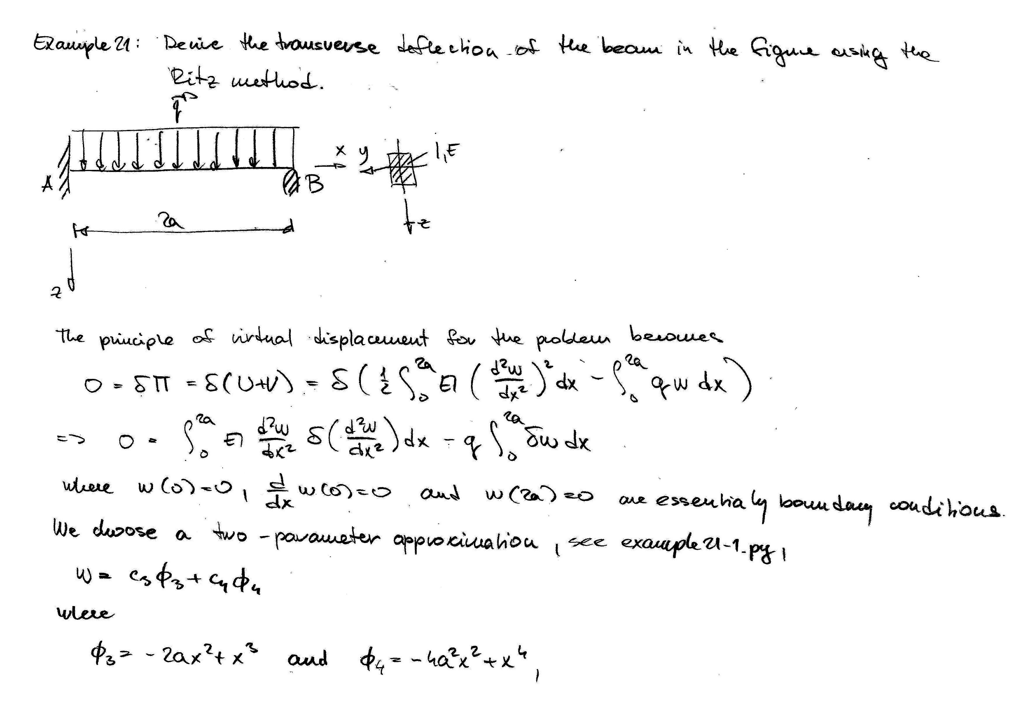
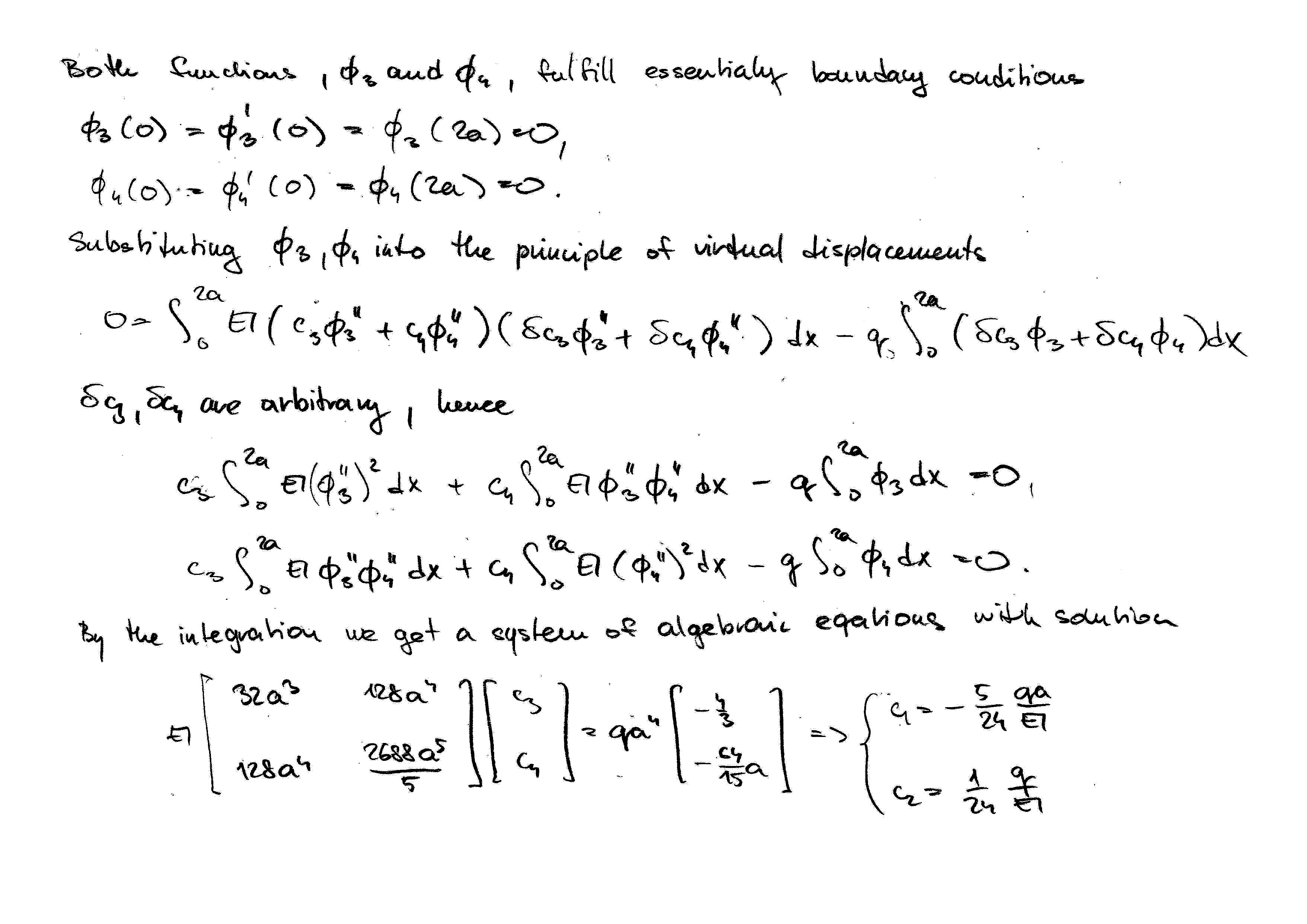
Ritz Method
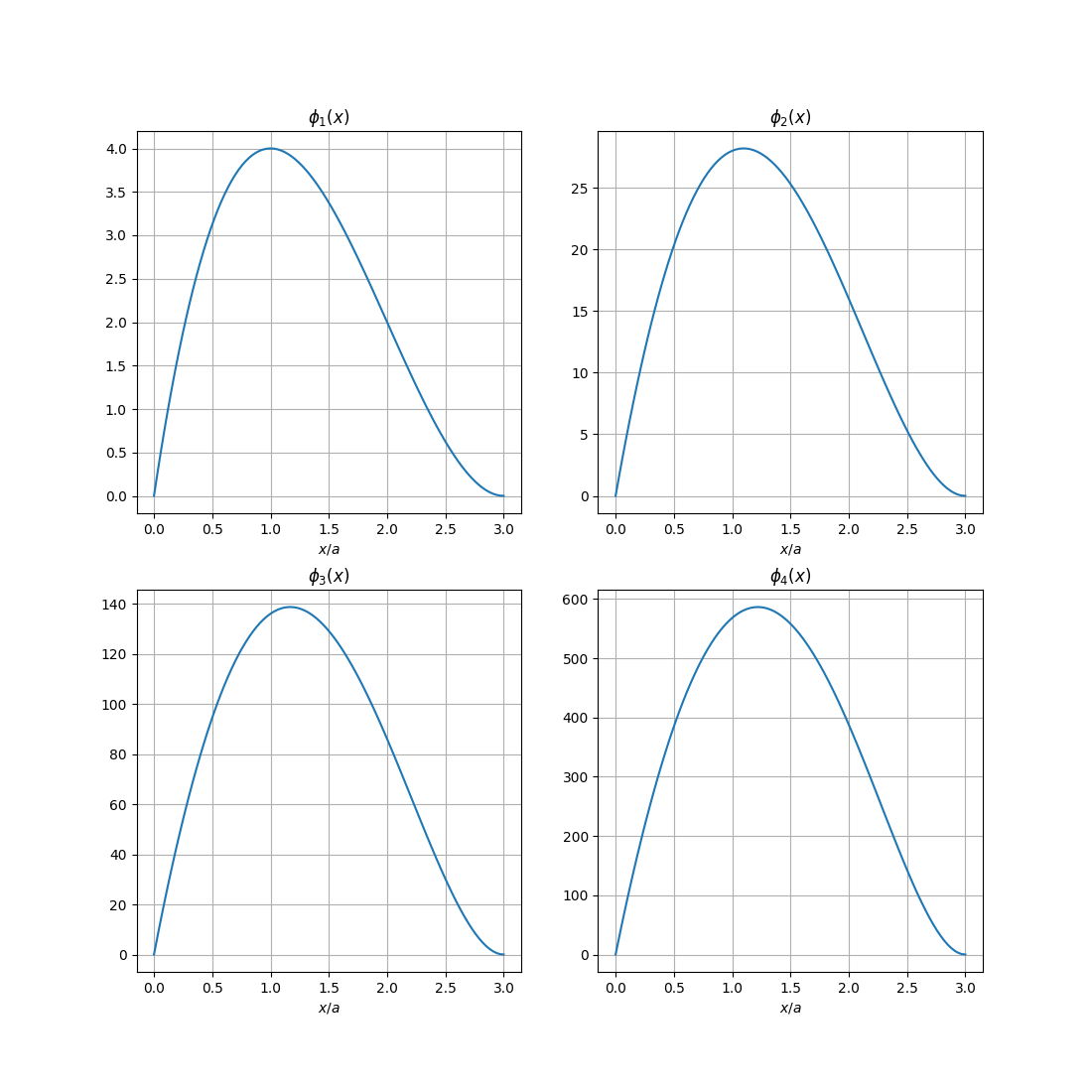
In the Ritz method, the displacements \(u_i\) for \(i=1,2,3\) are approximated by a finite combination of the form
where the parameters \(c_j^i\) must be determined by requiring that the principle of virtual displacements hold for arbitrary variations of these parameters. The functions \(\phi_0^i(x_k)\) and \(\phi_j^i(x_k)\) must satisfy the following requirements:
\(\phi_0^i(x_k)\) should satisfy the specified essential boundary conditions associated with \(u_i(x_k)\),
\(\phi_j^i(x_k)\) for \(j=1,2,\dots,n\) must be continuous as required by the variational principle being used,
\(\phi_j^i(x_k)\) for \(j=1,2,\dots,n\) satisfy the homogeneous form of the specified essential boundary conditions,
\(\phi_m^i(x_k)\) and \(\phi_n^i(x_k)\) must be linearly independent for \(m\neq n\) and \(m,n=1,2,\dots\),
\(\phi_j^i(x_k)\) must be complete for \(j=1,2,\dots\).
The functions \(\phi_j^i(x_k)\) for \(j=0,1,\dots\) form an infinite basis of the particular function space (a vector space in which vectors are replaced by functions) on some finite domain \(x_k\in \Omega\). The above mentioned combination of the requirements that these functions \(\phi_j^i(x_k)\) must be as complete and sufficiently smooth as the variational principle requires is generally very problematic from the mathematical point of view. It is a great achievement of modern mathematics that functional spaces satisfying this requirements was found for the wide range of partial differential equations used in mathematical physics.
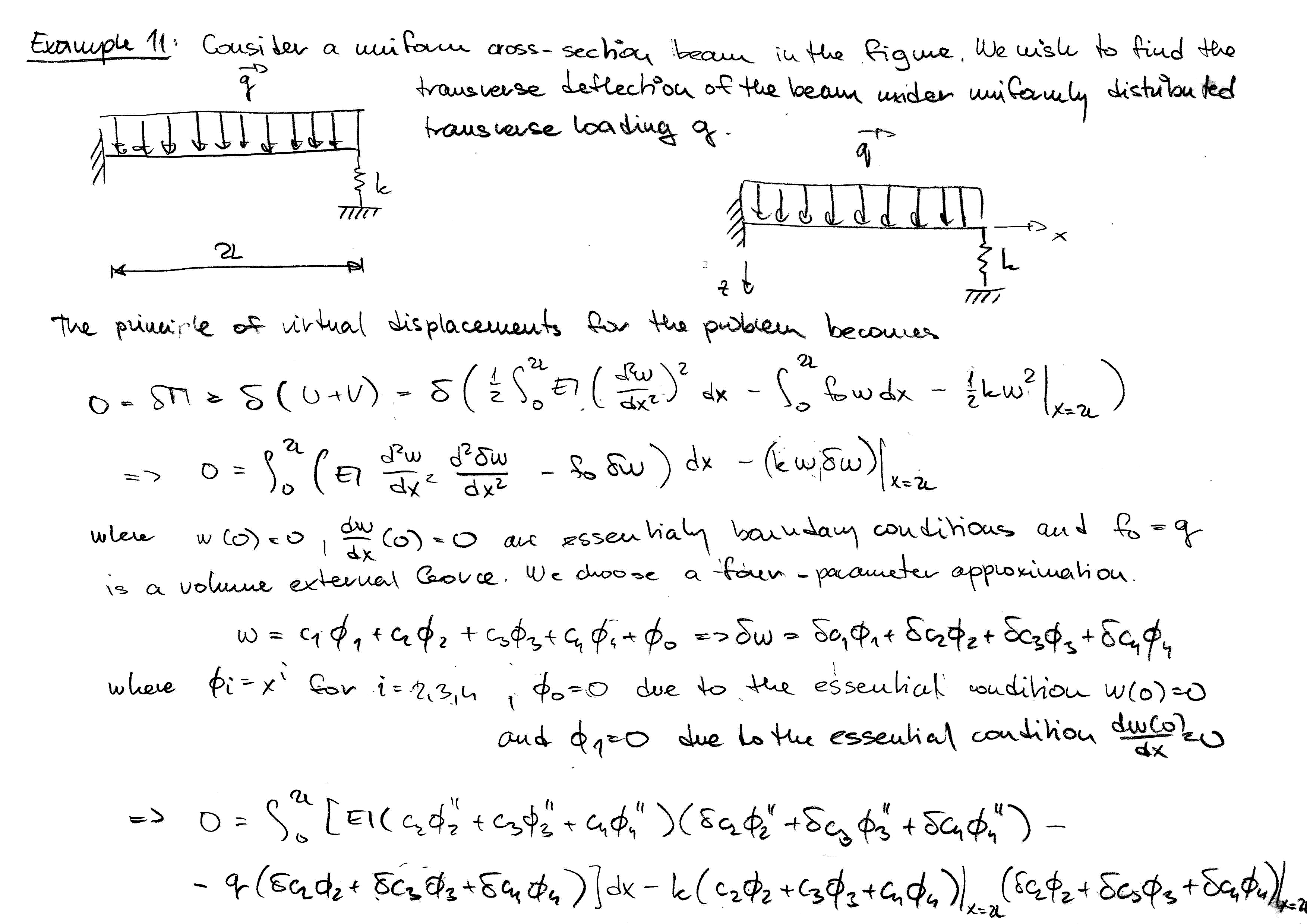
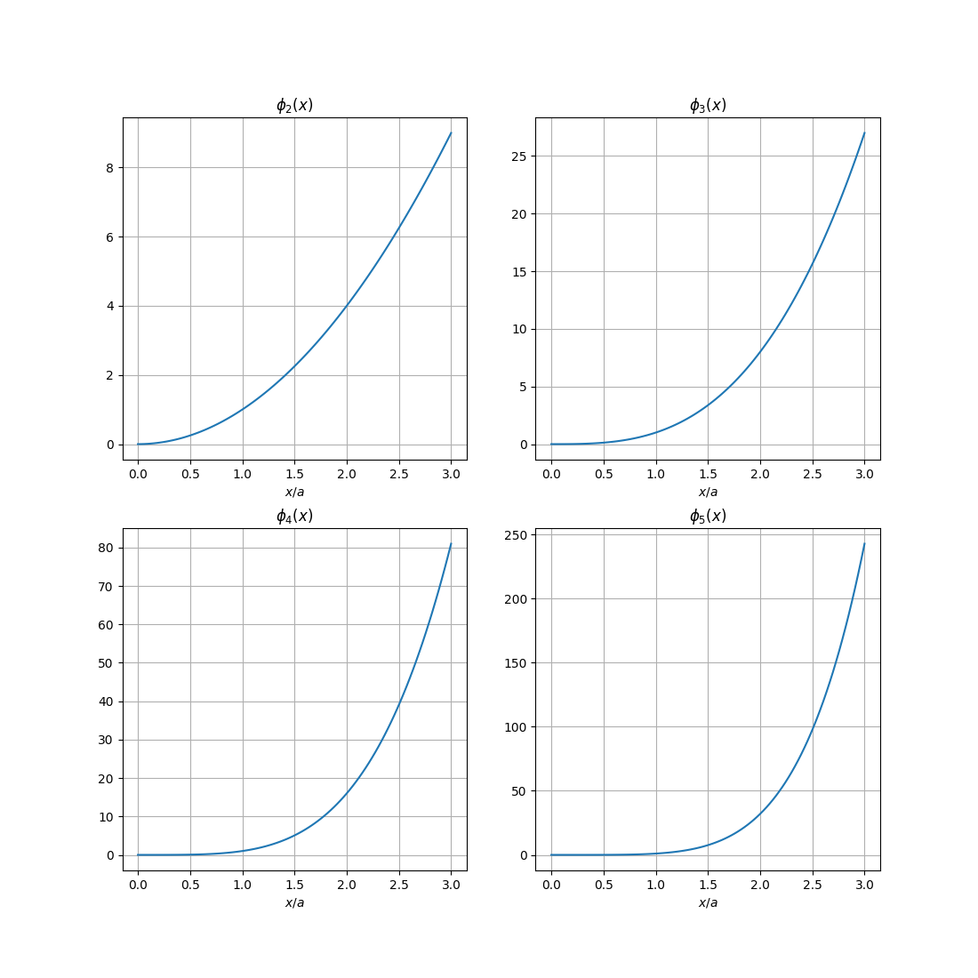
Since the natural boundary conditions of the problem are included in the variational statement, we require the assumed displacements \(U_i(x_k)\) to satisfy only the essential boundary conditions. For convenience, we select \(\phi_j^i(x_k)\) for \(j=1,2,\dots\) to satisfy the homogeneous form and \(\phi_0^i(x_k)\) to satisfy the actual form of the essential boundary conditions. The general rule is that the coordinate functions \(\phi_j^i(x_k)\) should be selected from an admissible set, from the lowest order to a desirable order, without missing any intermediate terms. The \(j\)-order components of the polynomials \(\phi_j^i(x_k)=x^j\) can be chosen in the case of the one-dimensional problems of the elasticity.
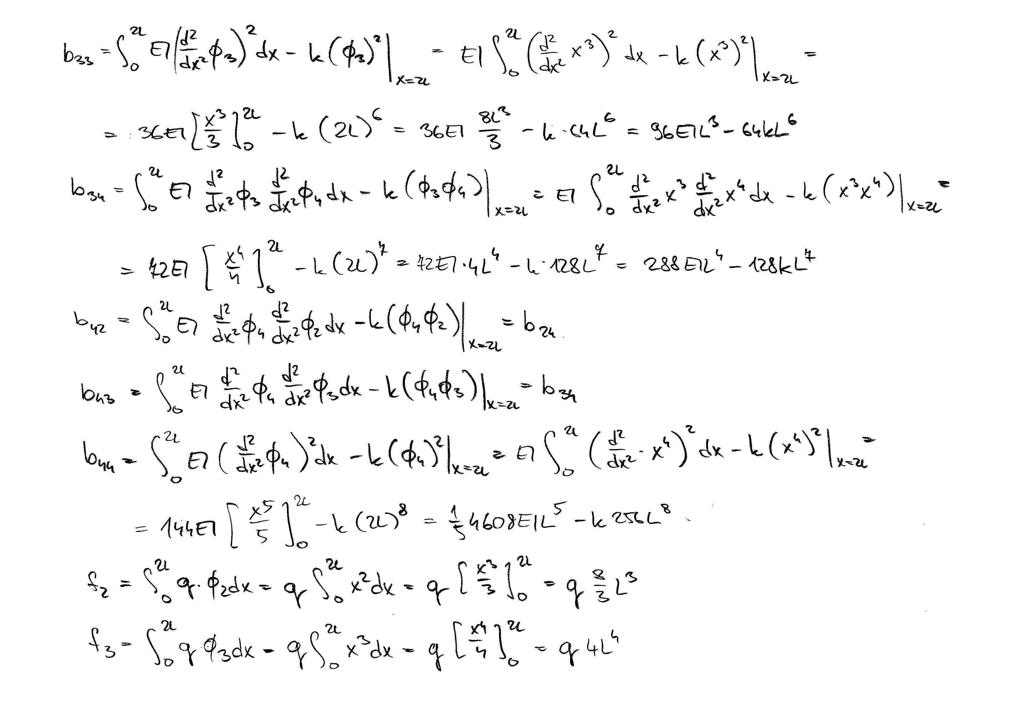
Equation (213) is used to compute approximate strains which are then used to compute the virtual work of the system in equilibrium given by the expression
We obtain
where the variation \(\delta u_i(x_k)\) were replaced by
Since \(\delta c_j^i\) for \(j=1,2,\dots,n\) are arbitrary and independent, it follows that
Thus, we obtain \(3n\) linearly independent simultaneous equations for the \(3n\) unknowns. Once \(c_j^i\) are determined from (217), the approximate displacements of the problem are given by (213). These displacements can be used to evaluate strains and stresses. Some general features of the Ritz approximations based on the principle of virtual displacements are as follows
for increasing values of \(n\), the previously computed coefficients of the algebraic equations (217) remain unchanged (provided the previously selected coordinate functions are not changed), and one must add newly computed coefficients to the system of equations,
if \(\delta\Pi\) is nonlinear in \(u_i\), the resulting algebraic equations will also be nonlinear in the parameters \(c_j^i\). To solve such nonlinear equations, a variety of numerical methods are available, such as the Newton-Raphson method, generally, there is more than one solution to the equations,
since the strains are computed from the approximate displacements, the strains and stresses are generally less accurate than the displacements,
the equilibrium equations of the problem are satisfied only in the energy sense \(\delta\Pi=0\), not in the differential equation sense, therefore the displacements obtained from the approximation generally do not satisfy the equations of equilibrium point-wise,
since a continuous system is approximate by a finite number coordinates (or degree of freedom), the approximate system is less flexible than the actual system, consequently, the displacements obtained by the Ritz method converge to the exact displacements from bellow, the displacements obtained from the Ritz approximations based on the complementary energy principle provide an upper bound for the exact solution.
The Ritz method is not applicable for the problems with complex geometry, external loadings and boundary conditions because it is not possible to establish the adequate function space, in which the solution should be found. On the other hand, the decomposition of the problem to be solved into the set of the simplified ones (elements) with respect to the geometry, loadings and boundary conditions allows the Ritz method to be used very effectively. This way of applying the Ritz method is known as the finite element method.
Examples 10:
Lecture 10 to download
hereas the pdf presentation.Example 10.1 to download
here,here,hereandhere. The auxiliary scripts in Python finding the basis functions and the solution of the Ritz method can be downloadedhereandhere, respectively. The graphs of basis functions and the solved beam deflection arehereandhere, respectively.Example 10.2 to download
here,here,hereandhere. The auxiliary scripts in Python finding the basis functions and the solution of the Ritz method can be downloadedhereandhere, respectively. The graphs of basis functions and the solved beam deflection arehereandhere, respectively.Example 10.3 to download
here,hereandhere. The auxiliary scripts in Python finding the basis functions and the solution of the Ritz method can be downloadedhereandhere, respectively. The graphs of basis functions and the solved beam deflection arehereandhere, respectively.