Výuka

PPI: zde a zde.

BKP Projekt

Má snad někdo dojem, že být Bakalářem je procházka rajskou zahradou? Zlatý voči! Je to život plný ústrků, ponižování a bezpráví, Kočka by svých devět životů za tenhle jeden mizerný nevyměnila. Jednoduše řečeno, je to život pod Psa. Více zde, teda pardon, támhle níž:

https://www.profant.cz/tomas_bkp.html#bkp.

Kinematika

  • Poznámka: Na vlastní nebezpečí, zvýšené riziko mozkové příhody.
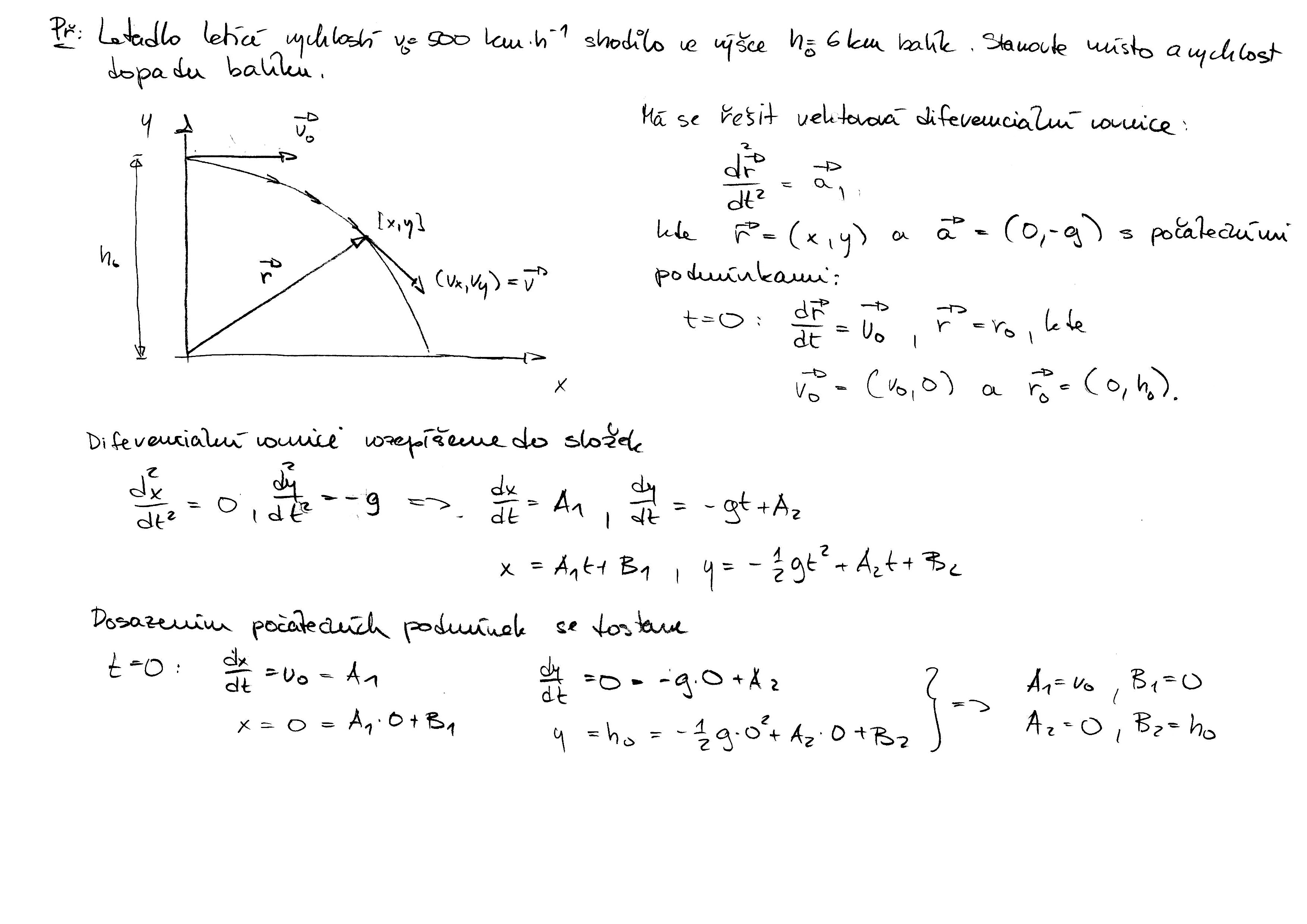
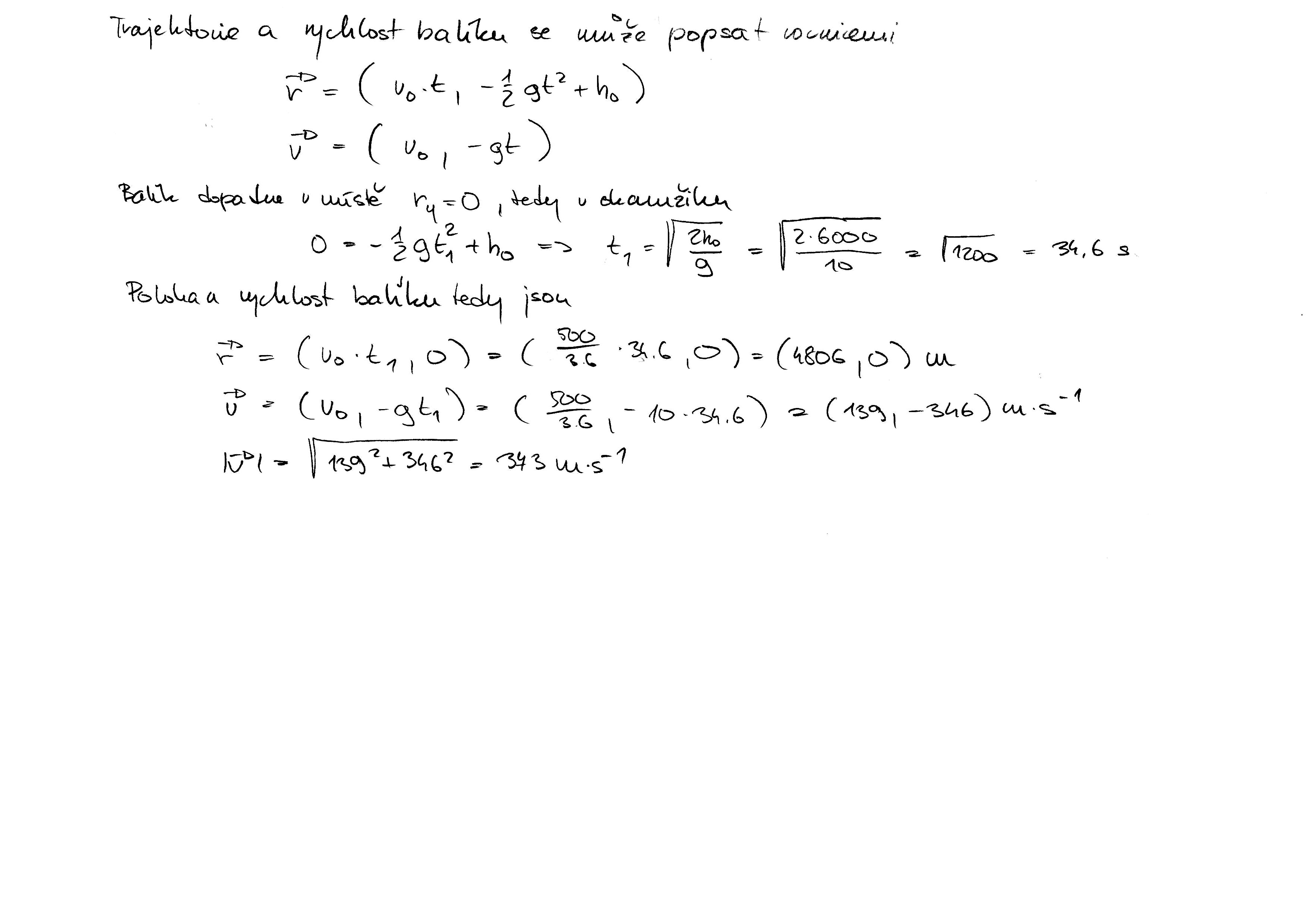
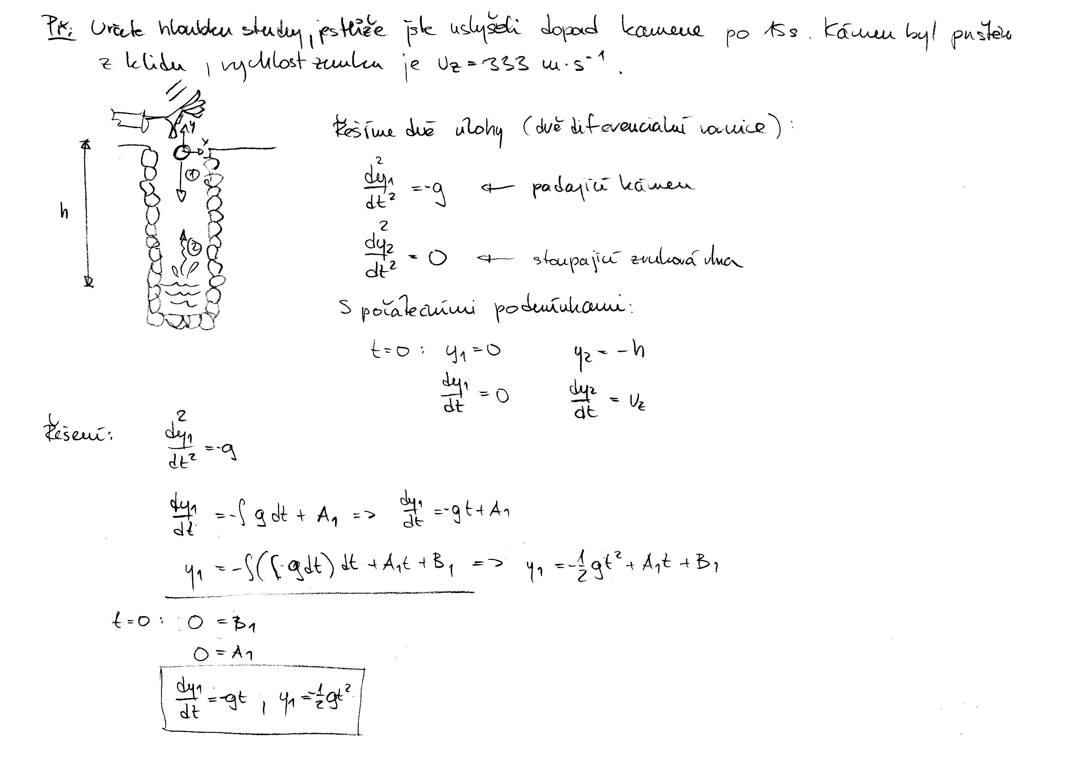
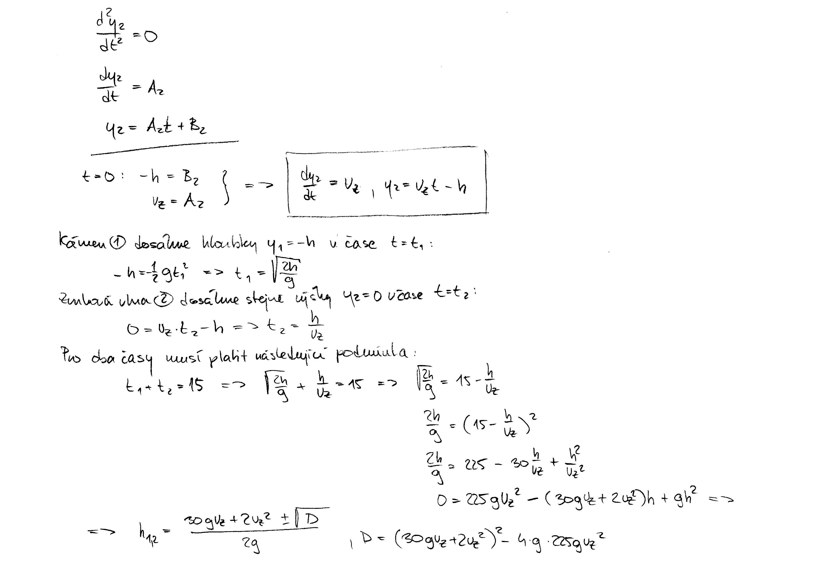
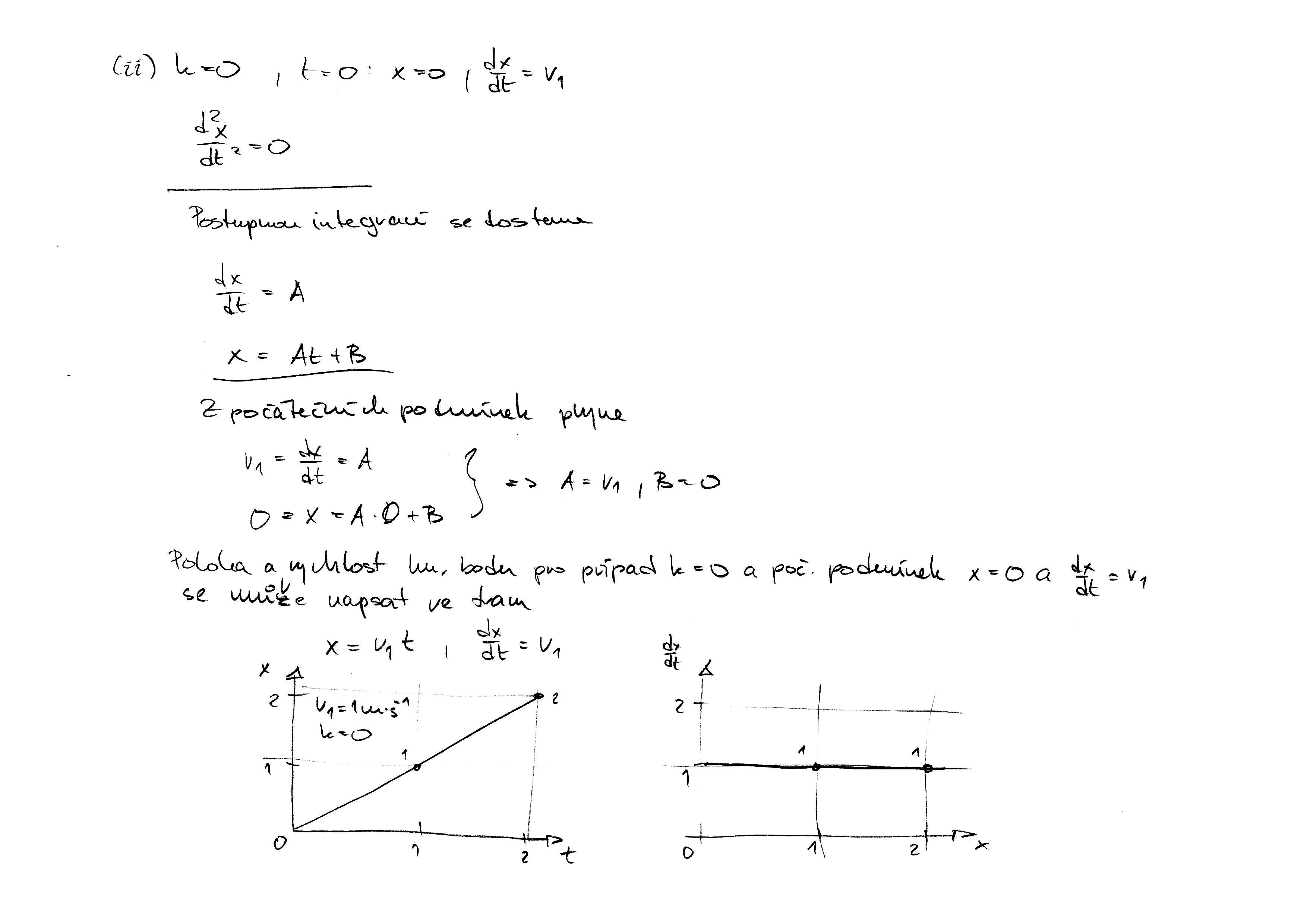
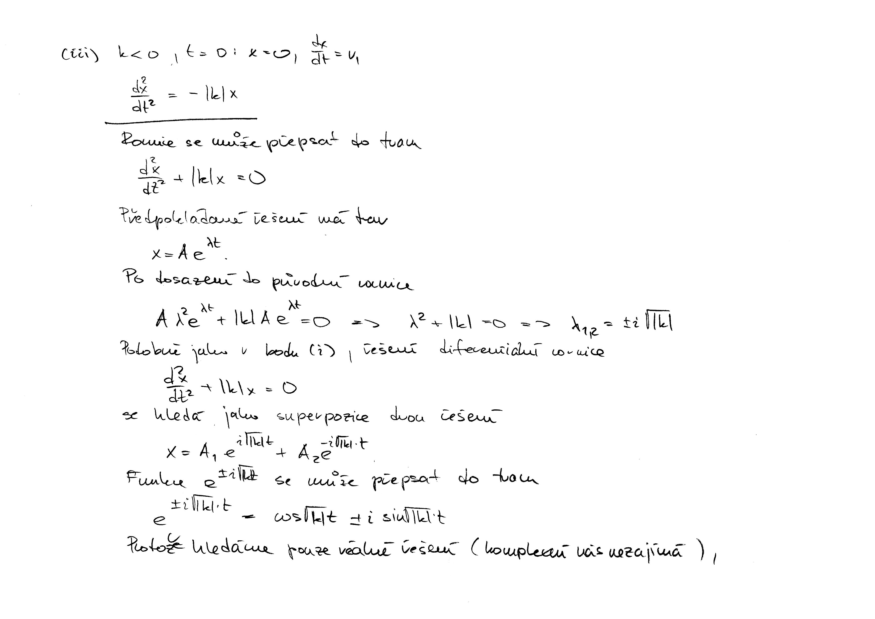
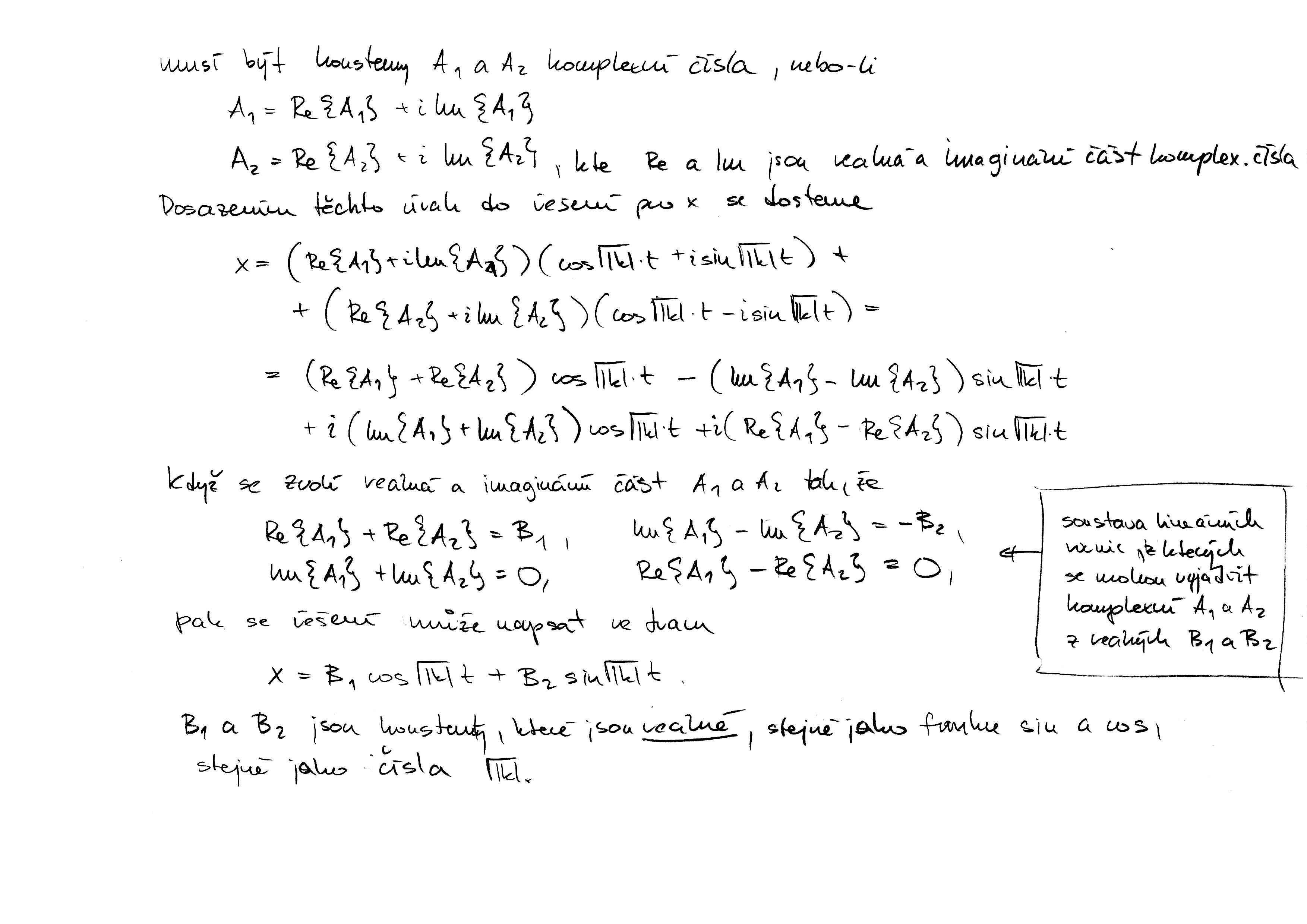
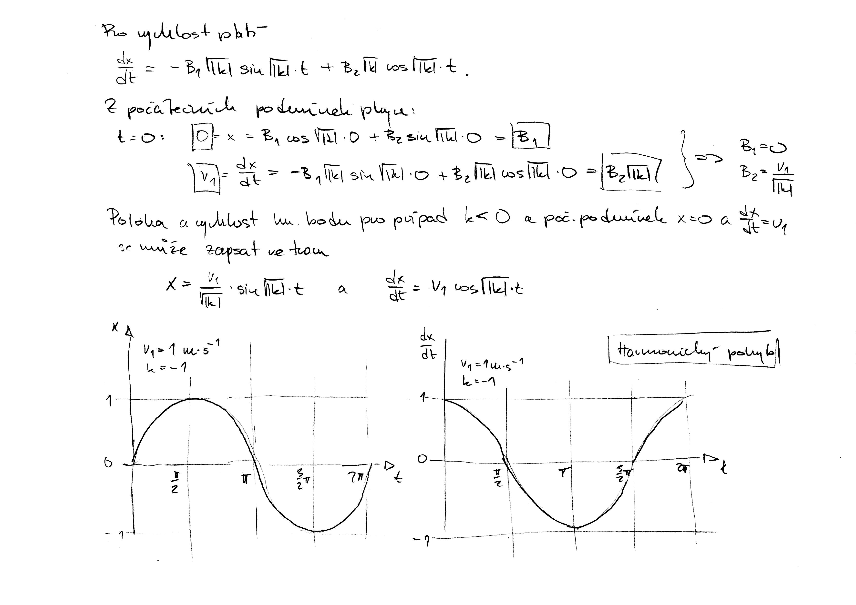
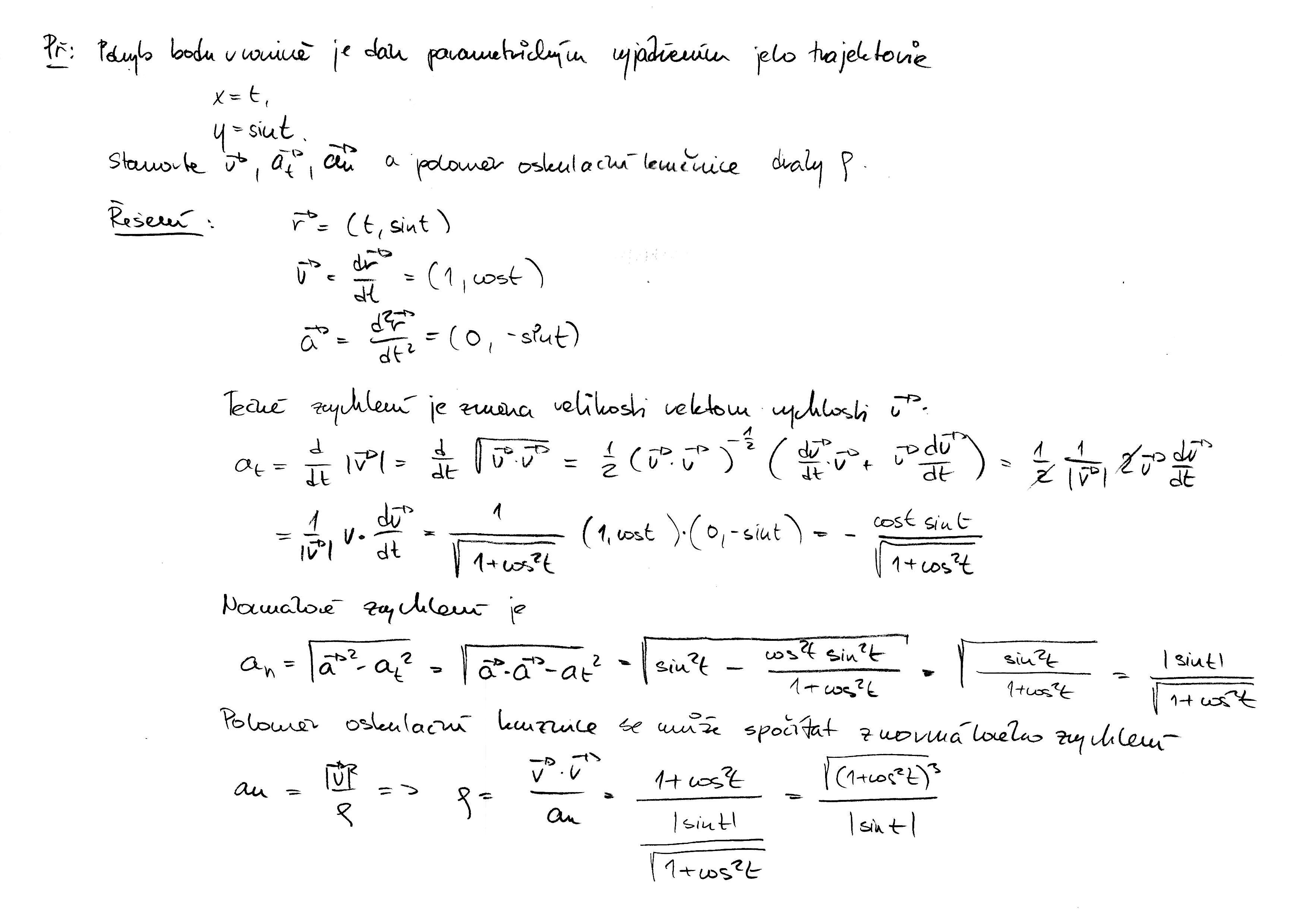
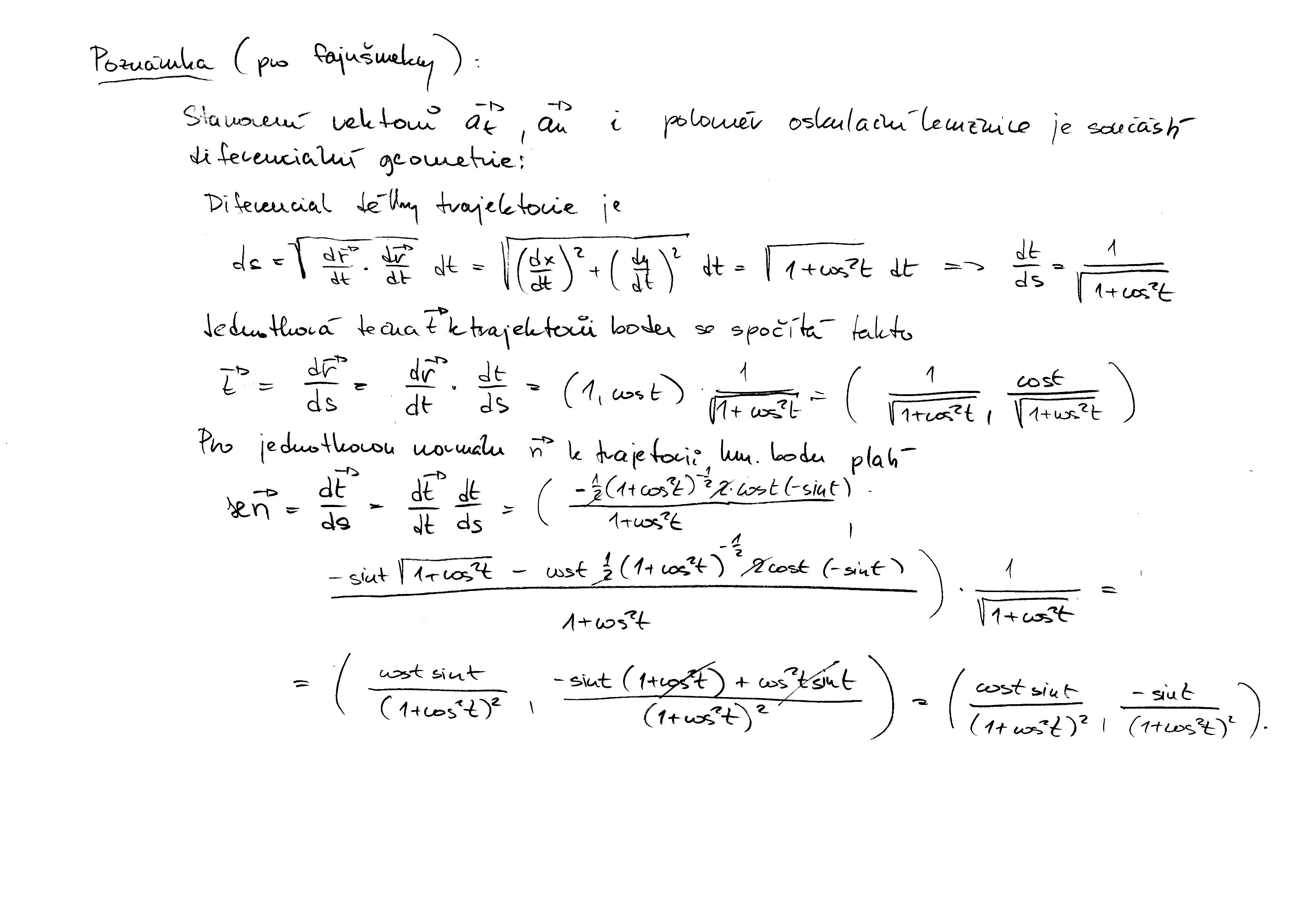
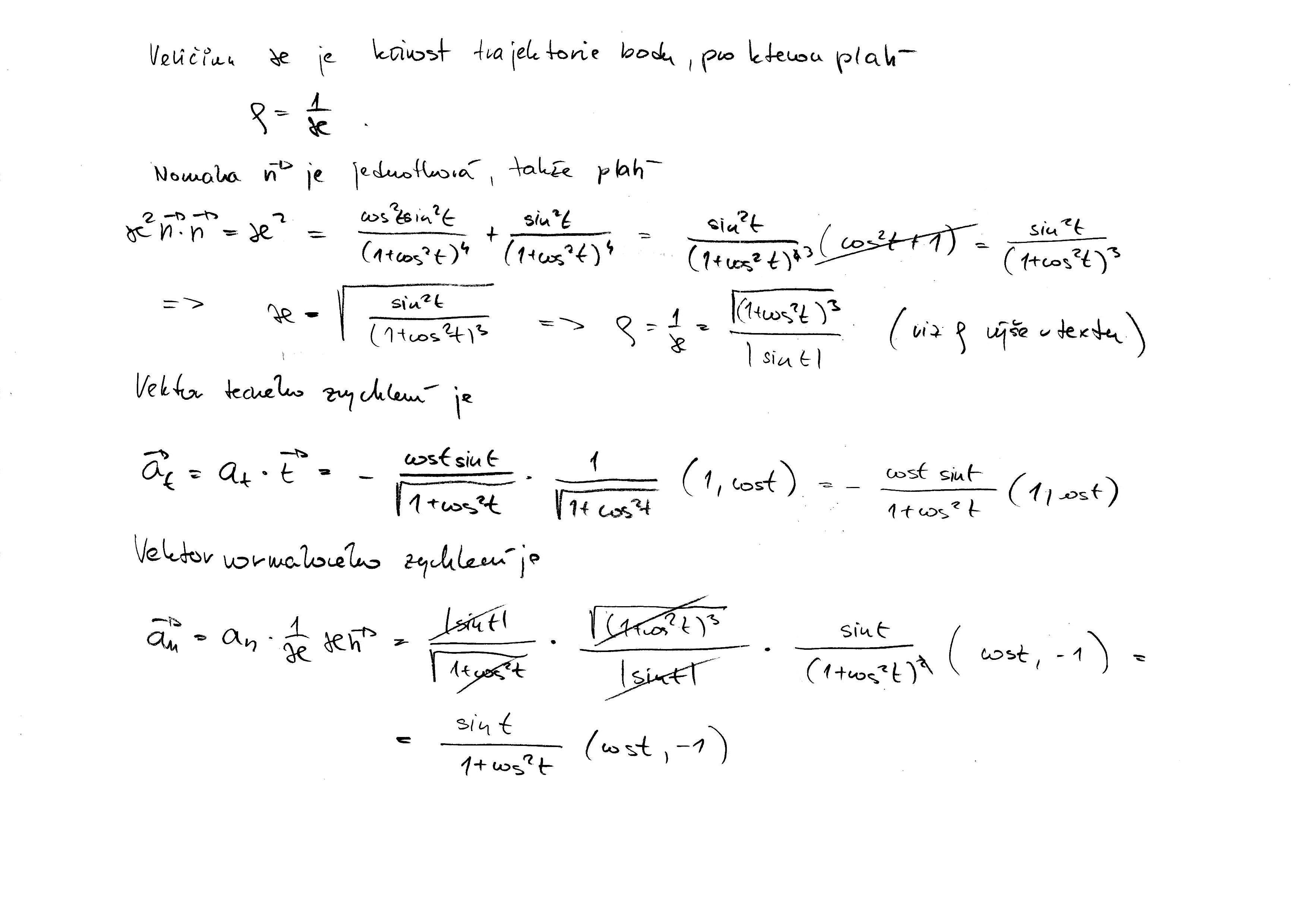
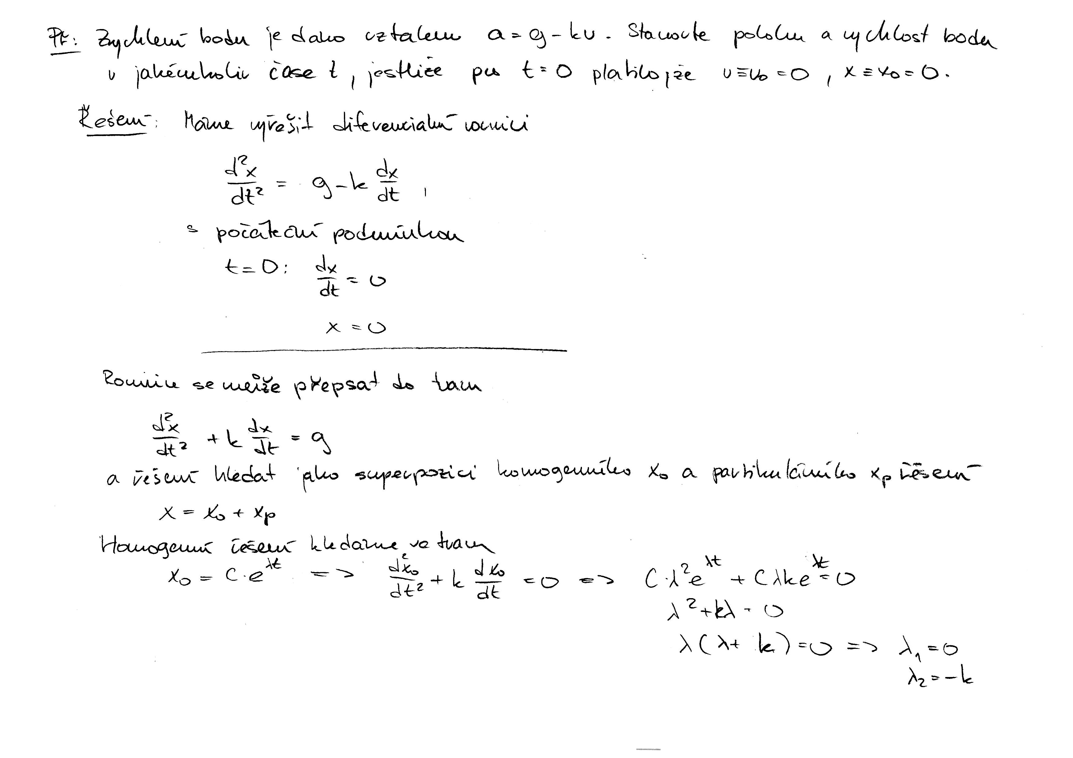
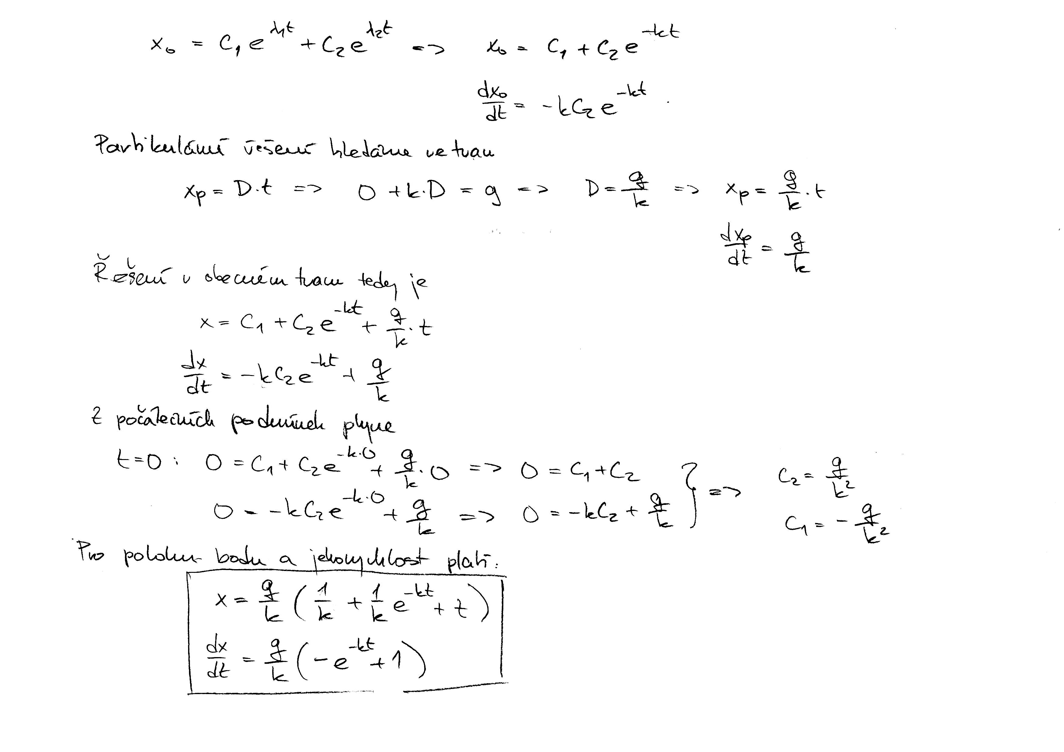
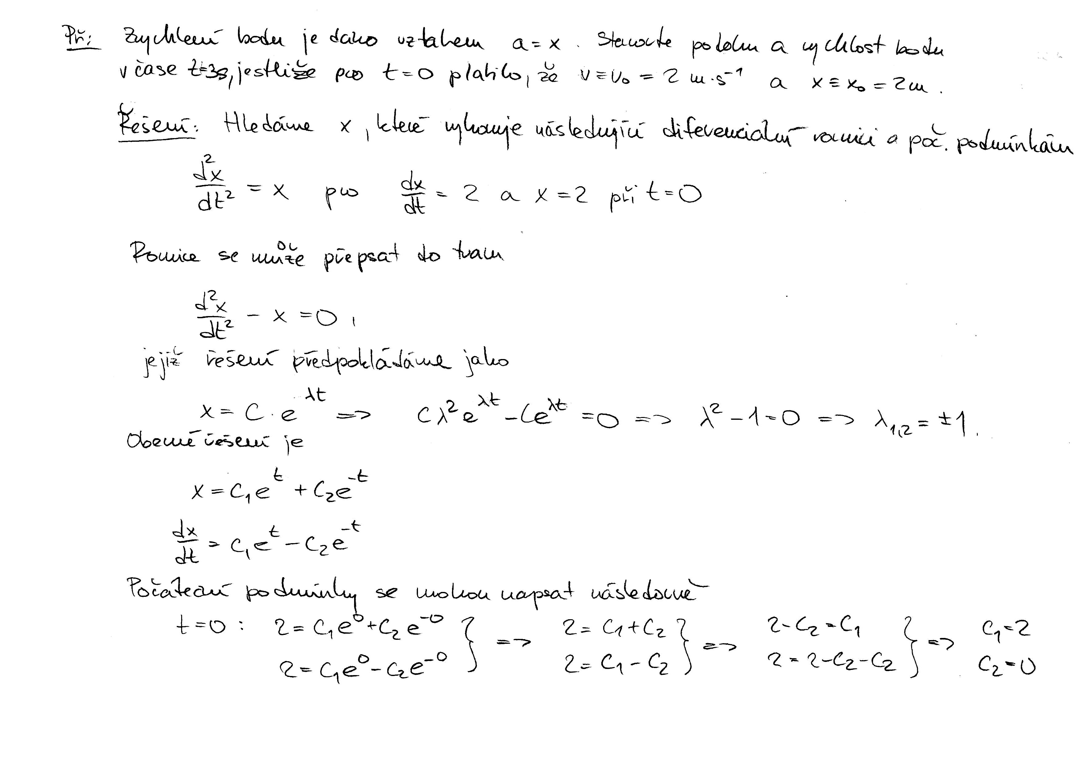
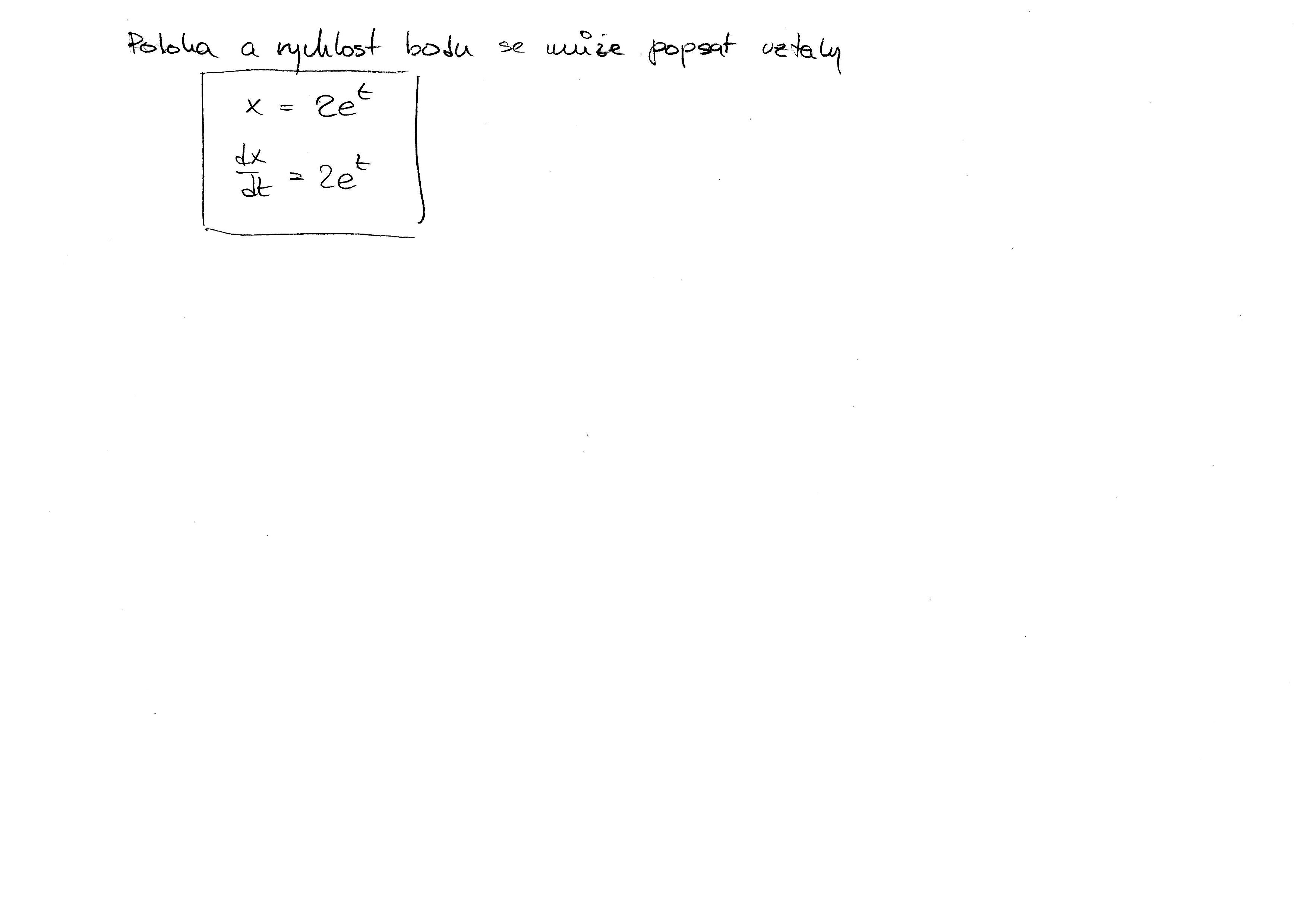
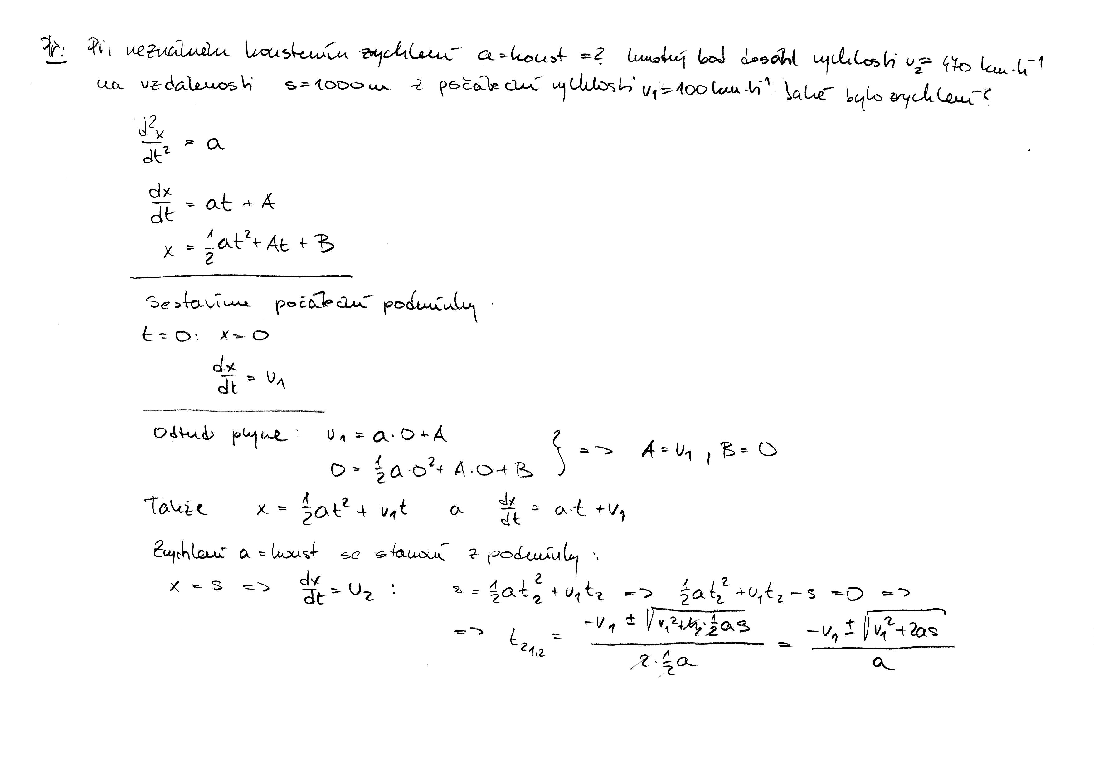
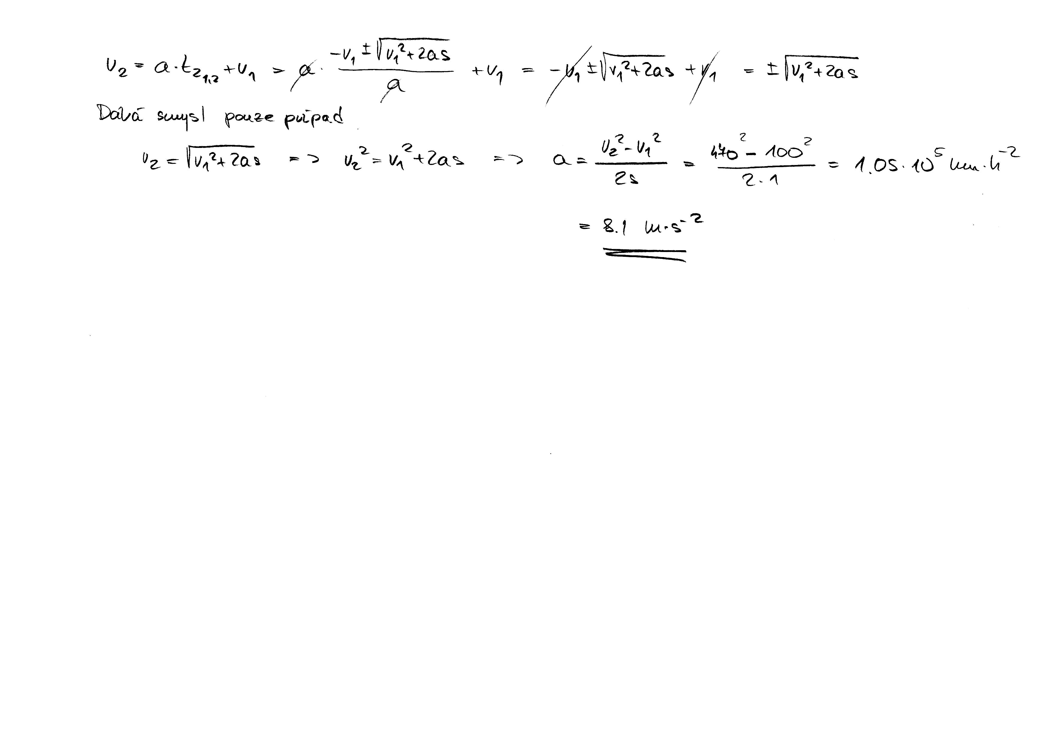
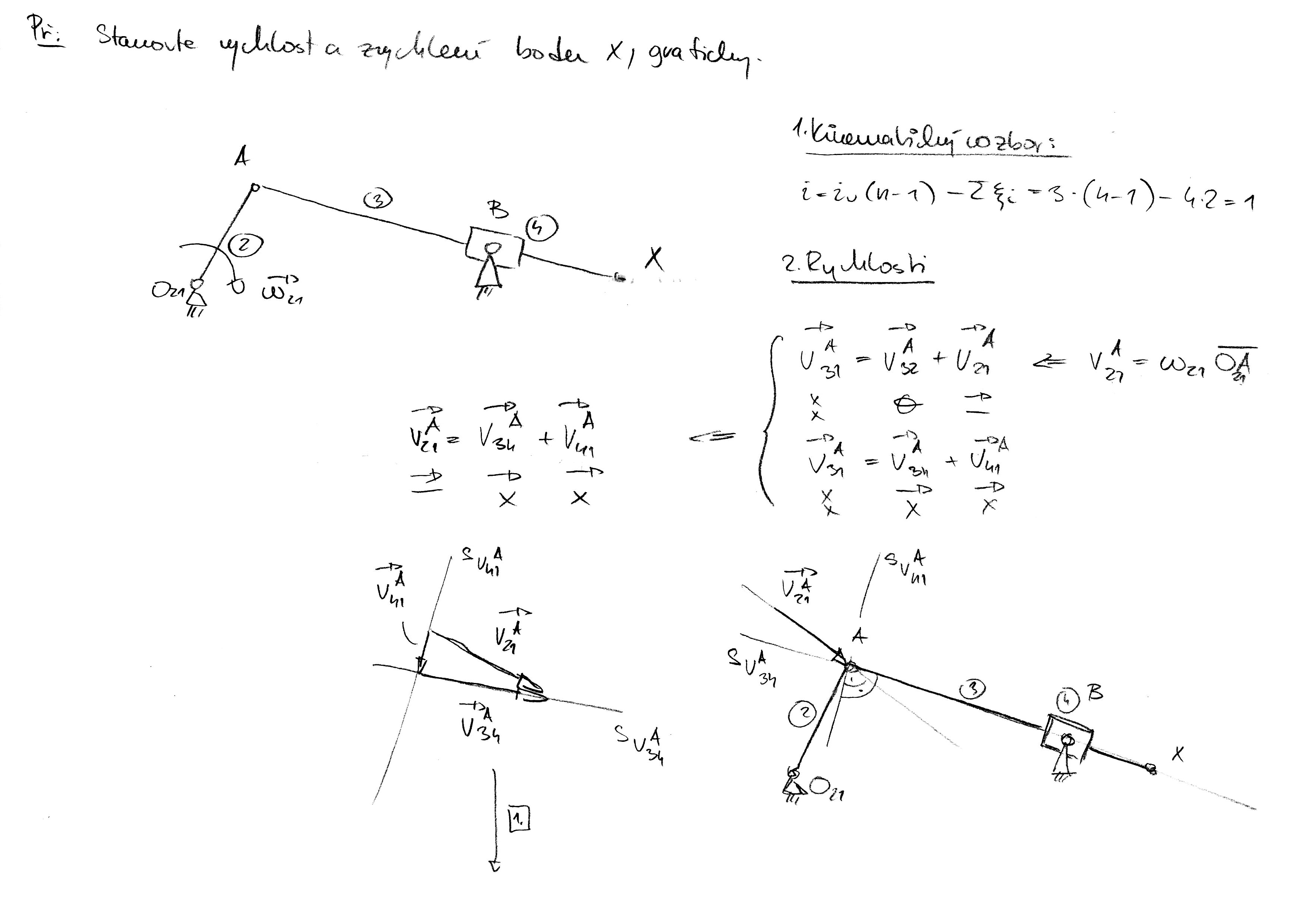
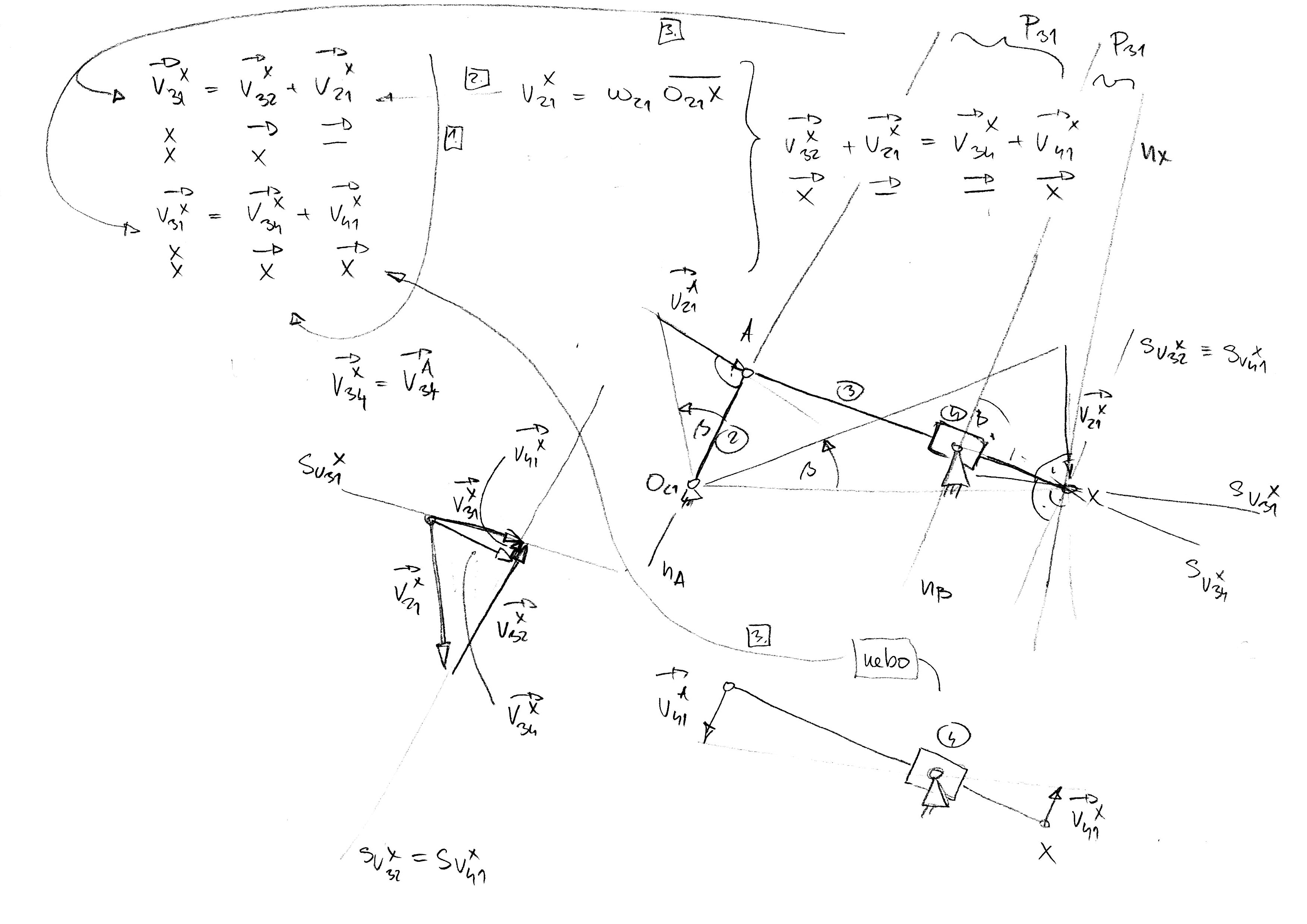
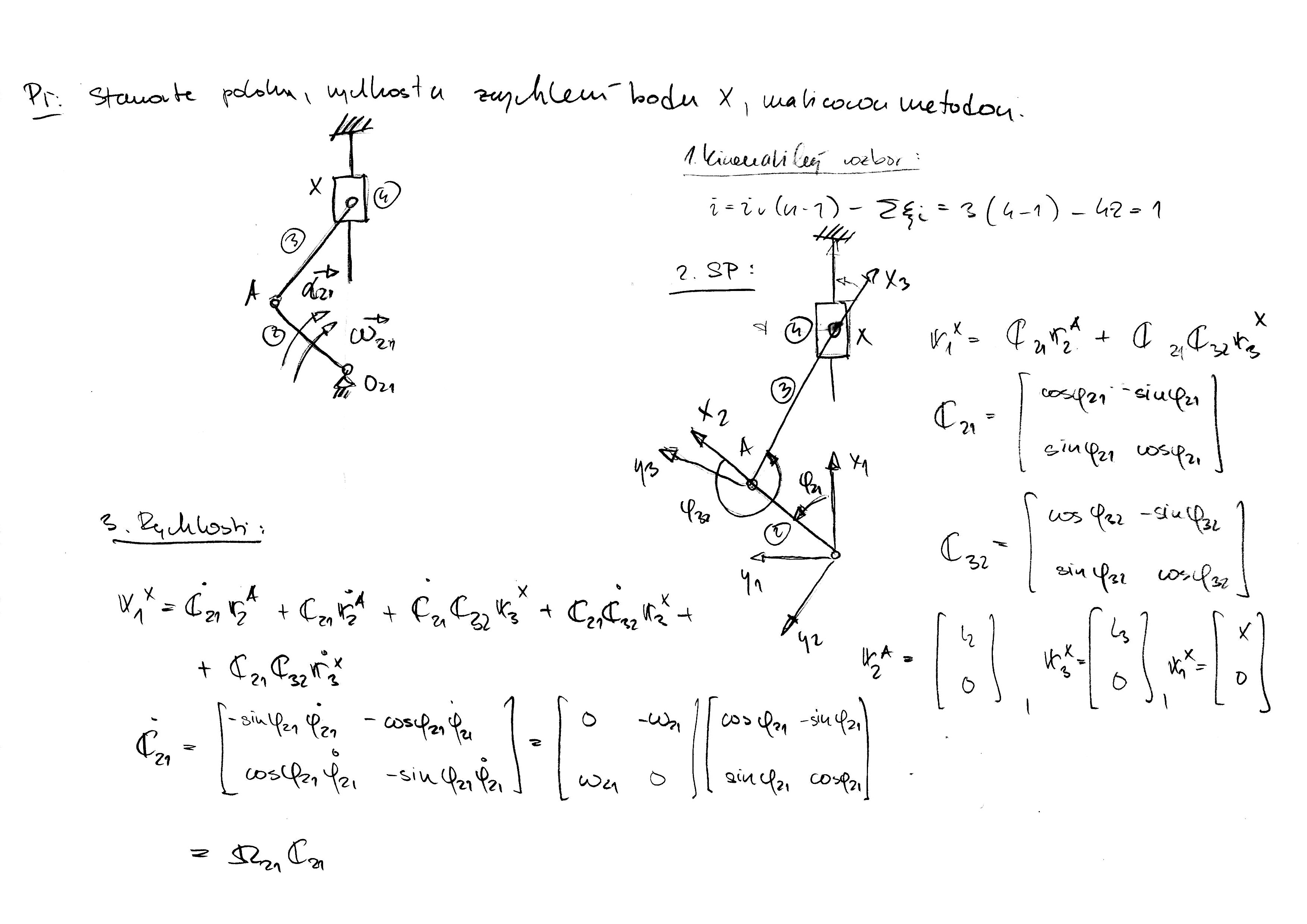
  • Cvičení 1: Kinematika bodu, vztahy mezi kinematickými veličinami.

    • Ručně řešený příklad Př.1 lze stáhnout zde a zde.

    • Ručně řešený příklad Př.2 lze stáhnout zde, zde a zde.

    • Ručně řešený příklad Př.3 lze stáhnout zde.

    • Ručně řešený příklad Př.4 lze stáhnout zde a zde.

    • Ručně řešený příklad Př.5 lze stáhnout zde a zde.

    • Ručně řešený příklad Př.6 lze stáhnout zde a zde.

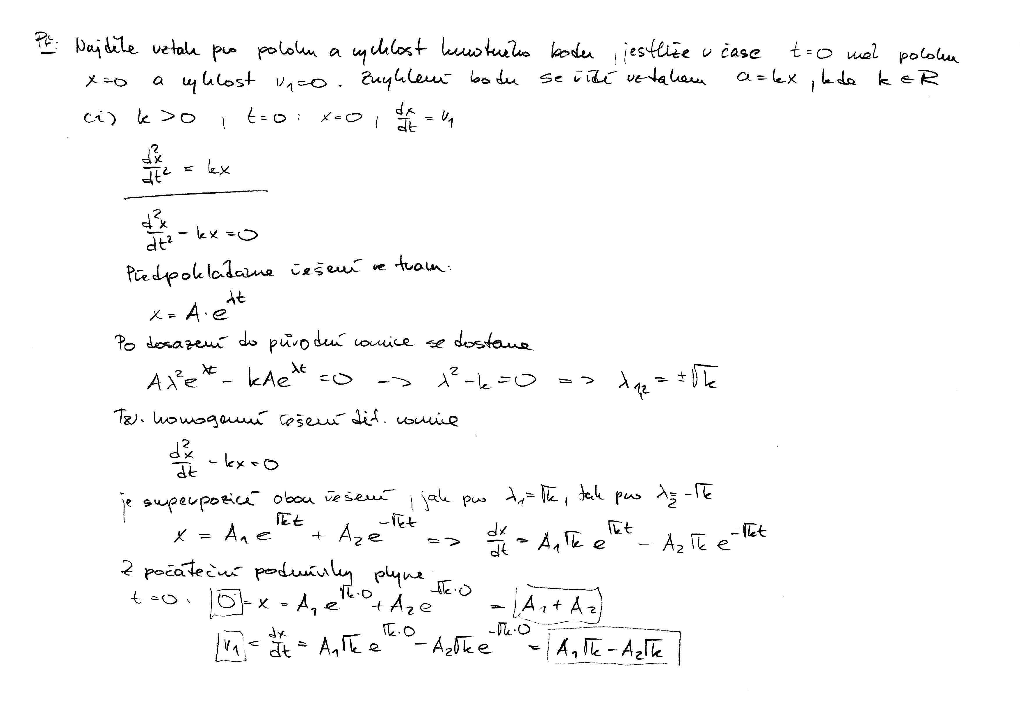
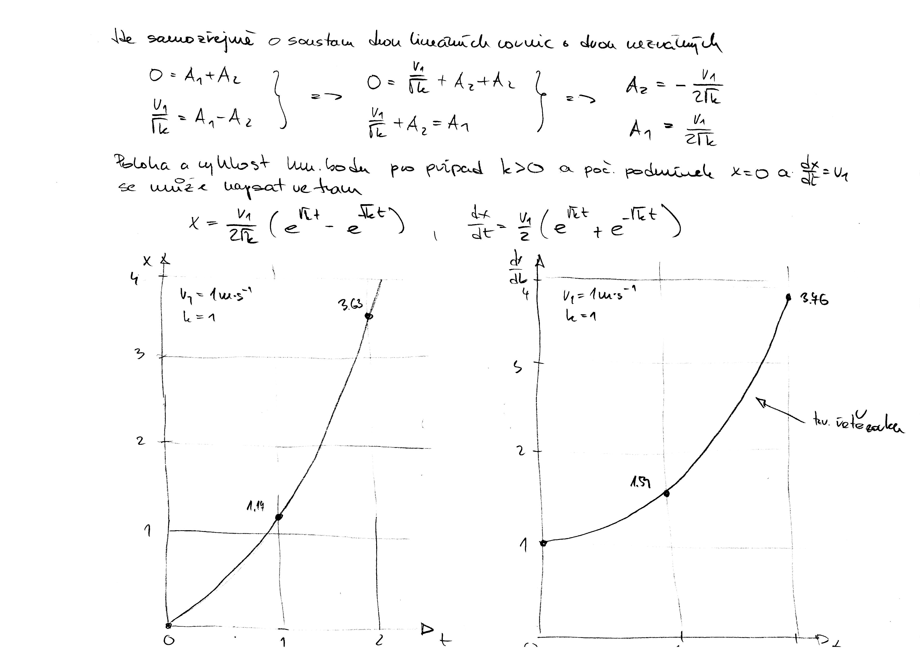
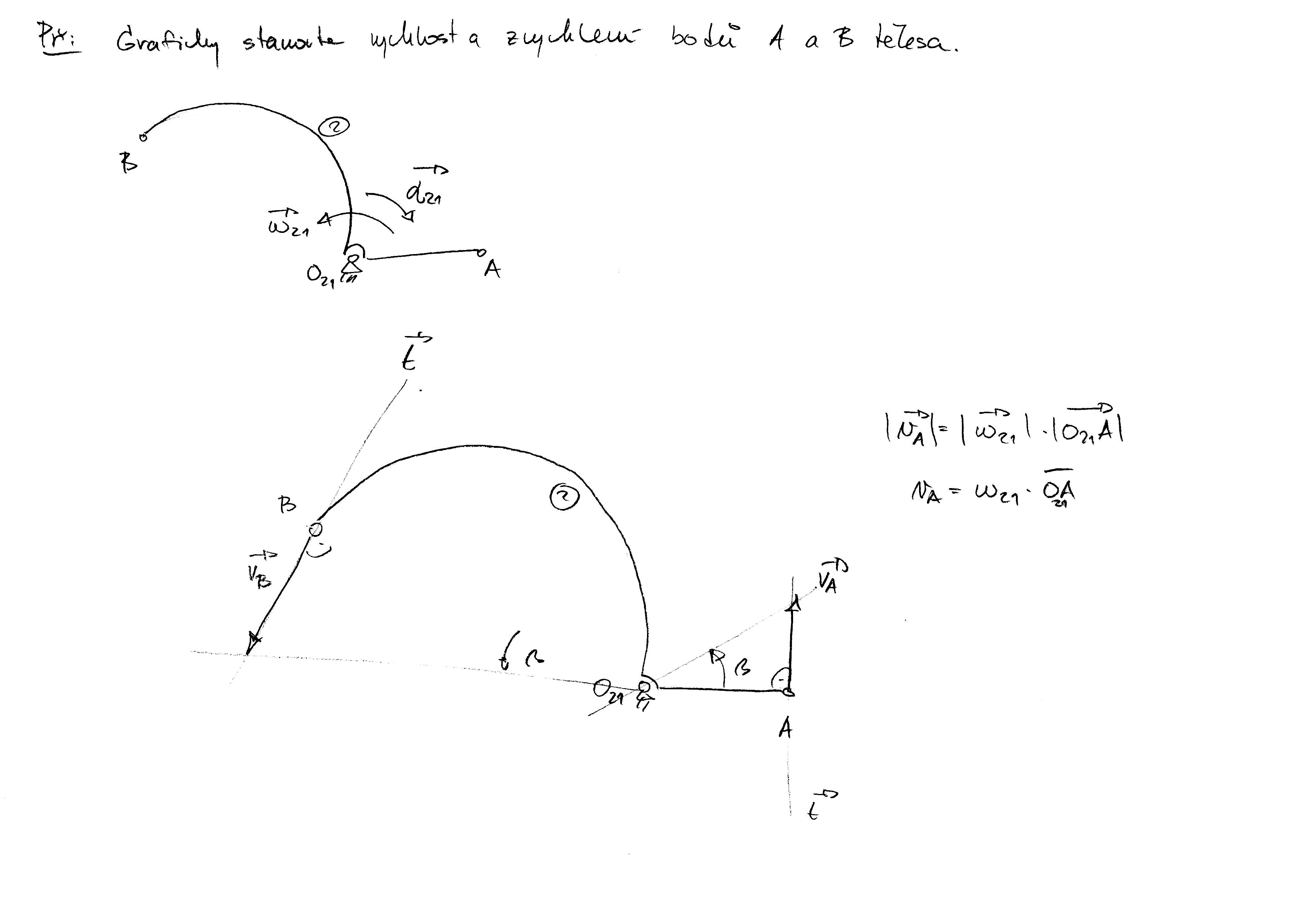
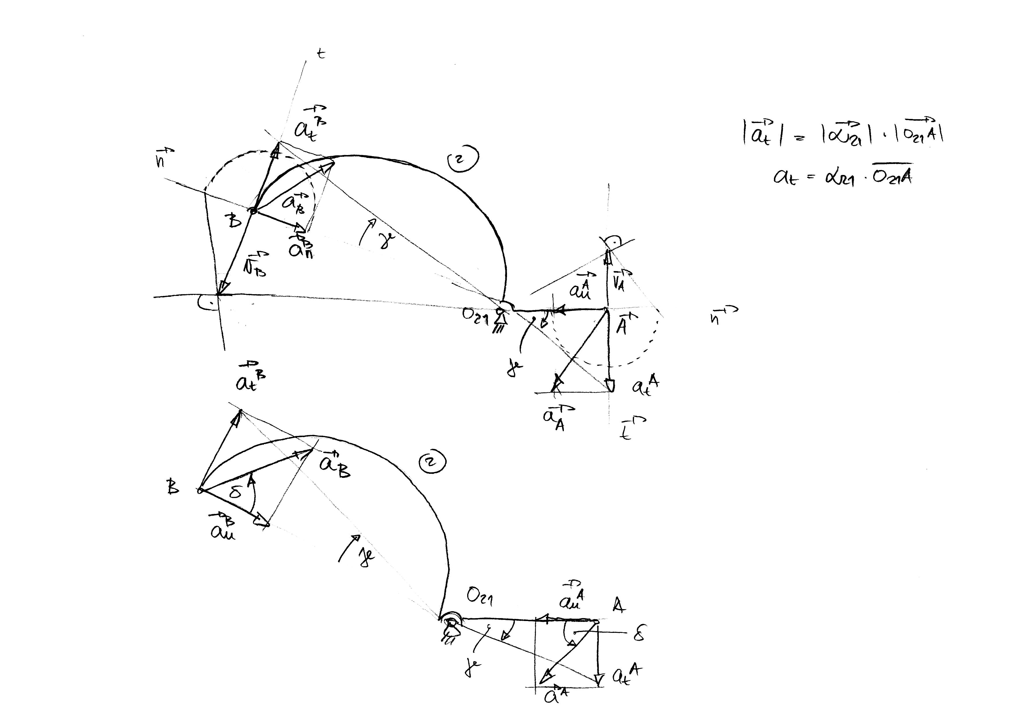
  • Cvičení 2: Kinematika bodu, střed křivost trajektorie.

    • Ručně řešený příklad Př.1 lze stáhnout zde a zde.

    • Ručně řešený příklad Př.2 lze stáhnout zde, zde, zde, zde, zde a zde.

    • Ručně řešený příklad Př.3 lze stáhnout zde a zde.

    • Ručně řešený příklad Př.4 lze stáhnout zde a zde.

    • Ručně řešený příklad Př.5 lze stáhnout zde, zde a zde.

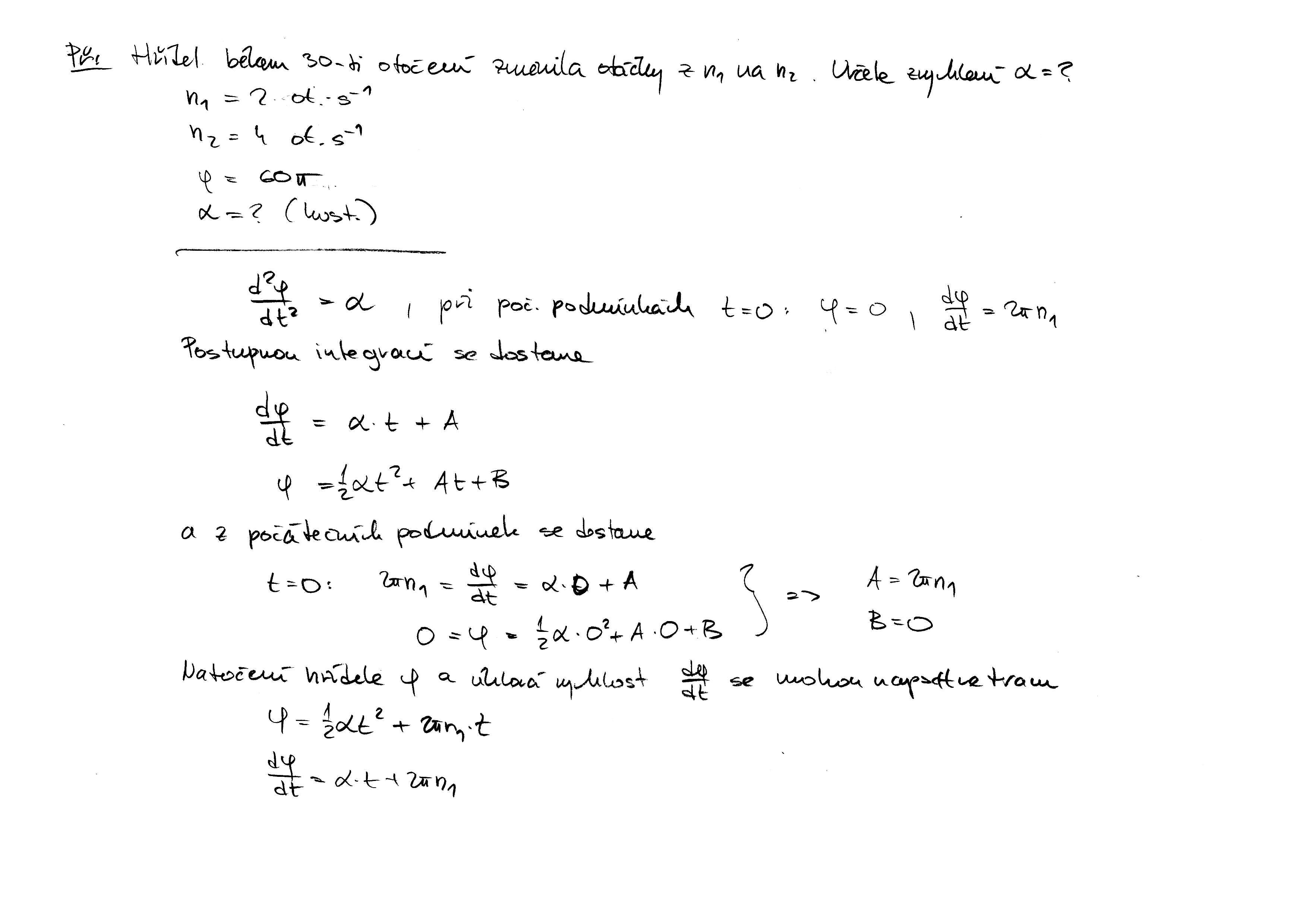
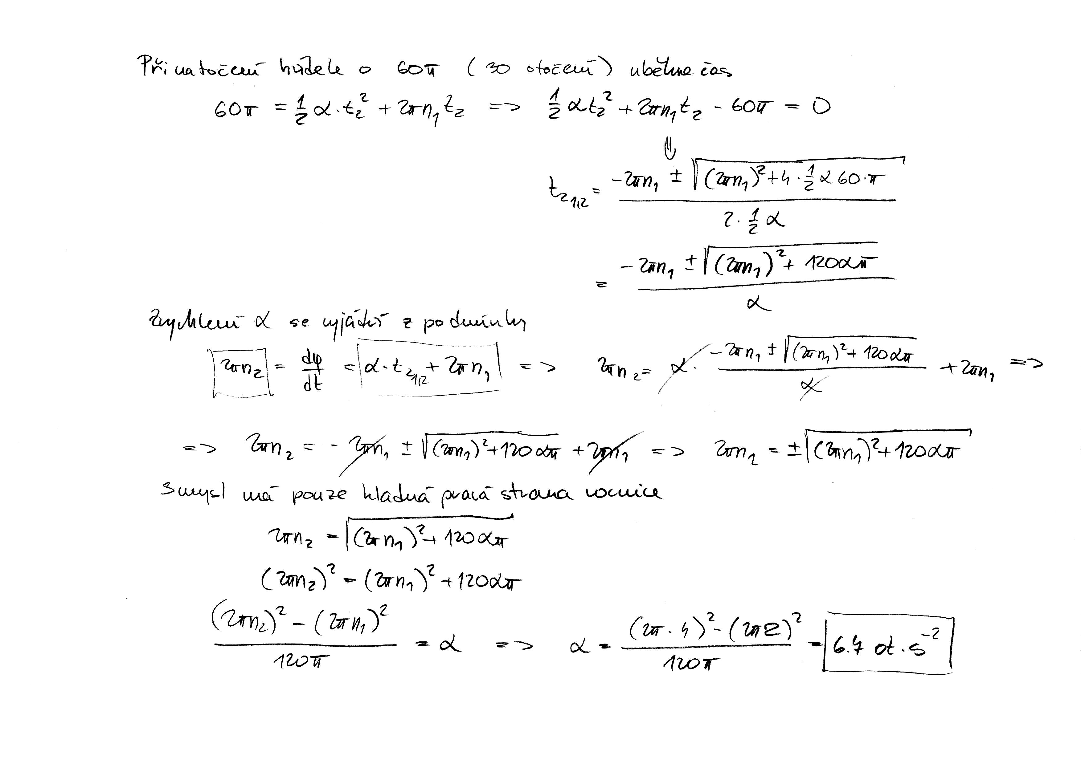
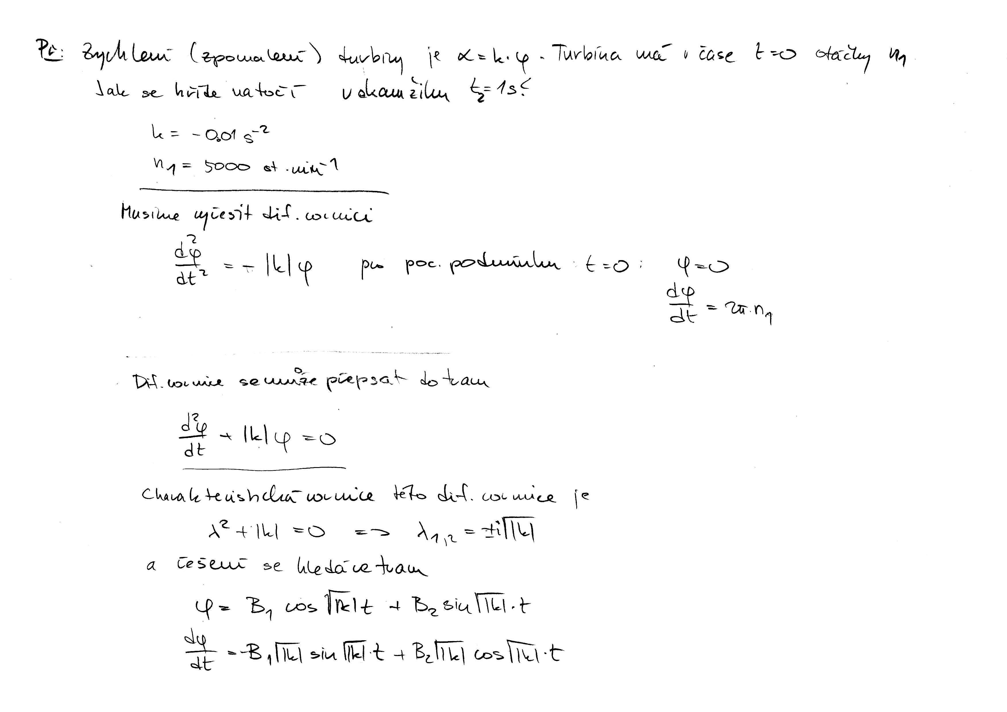
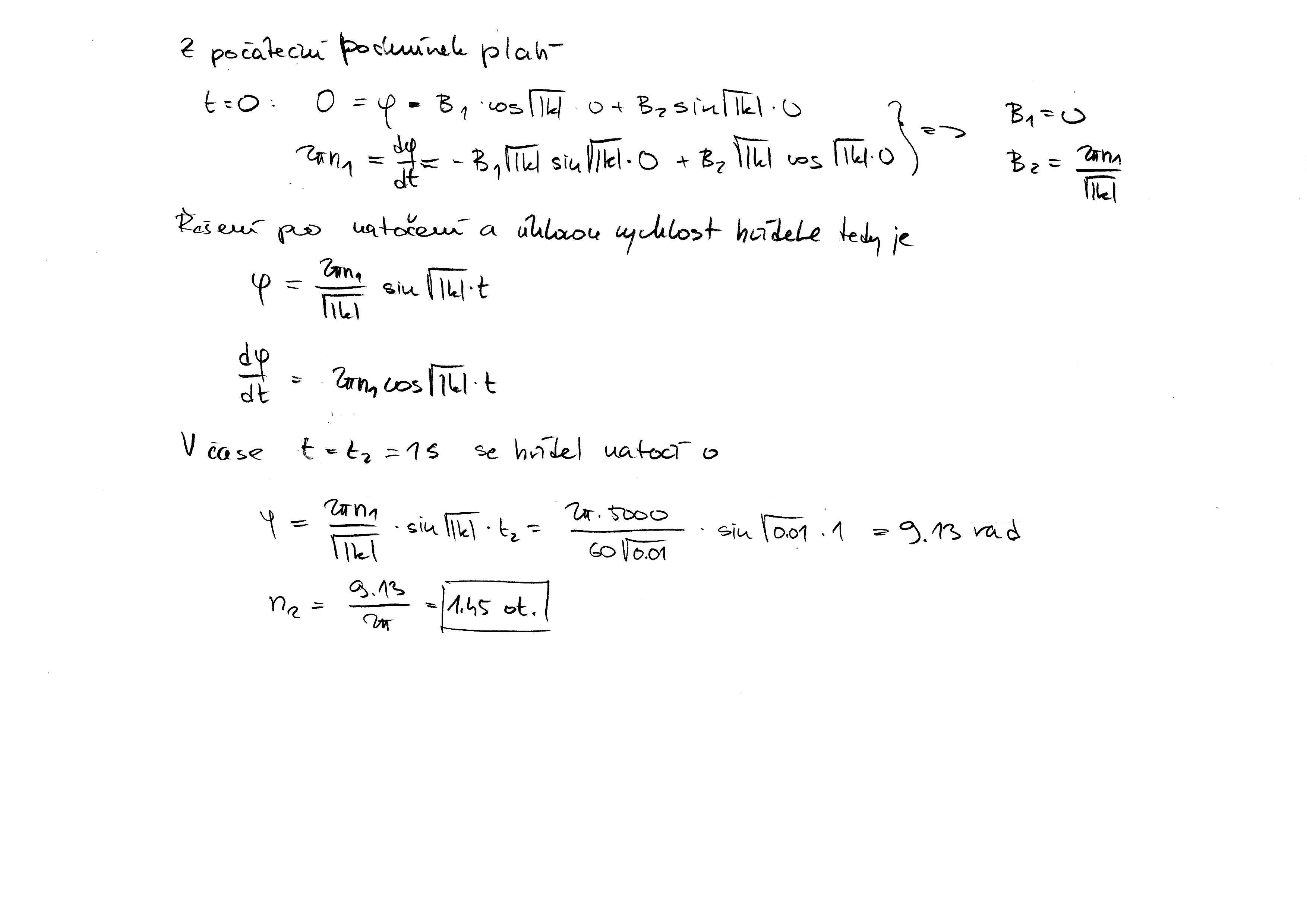
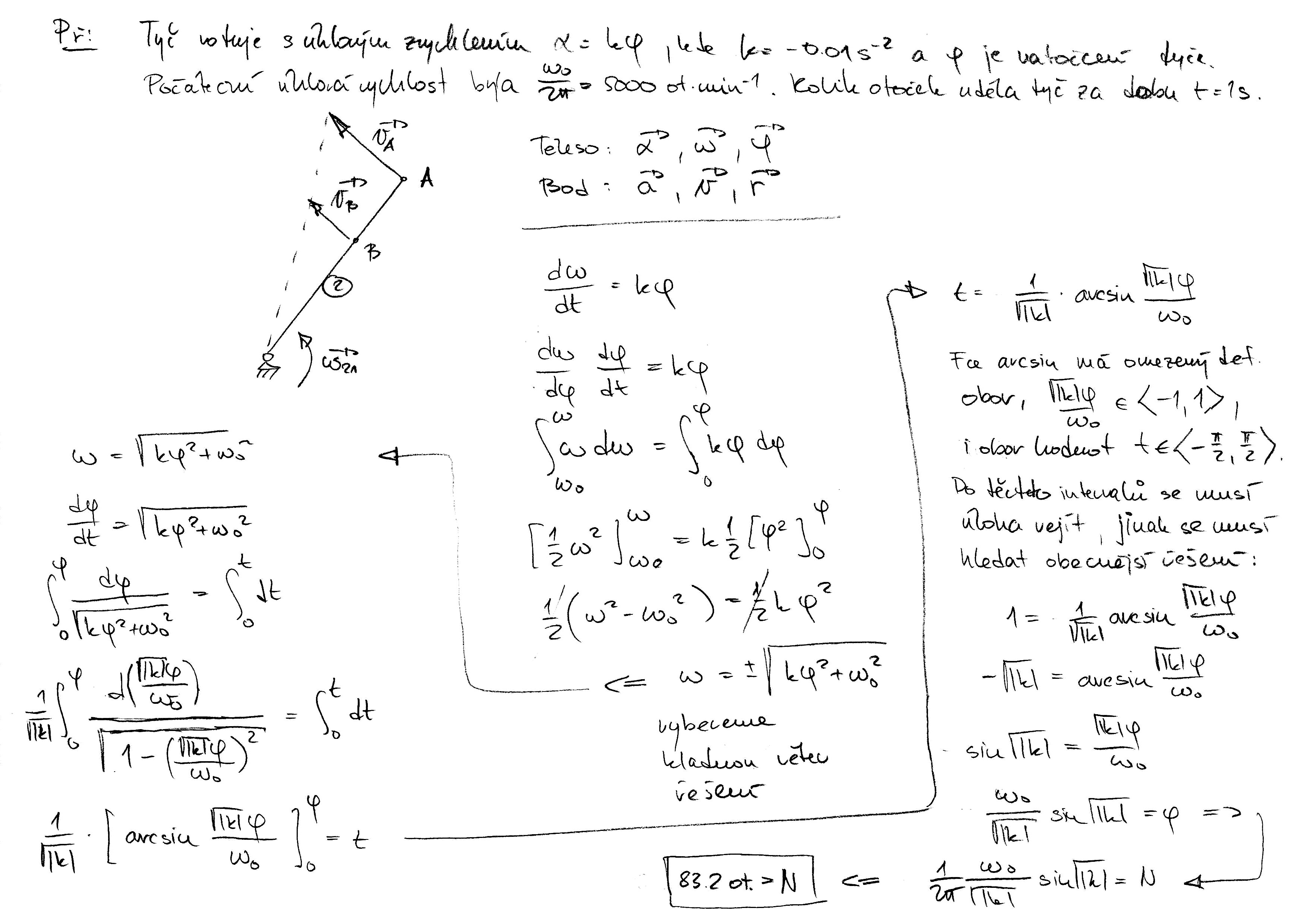
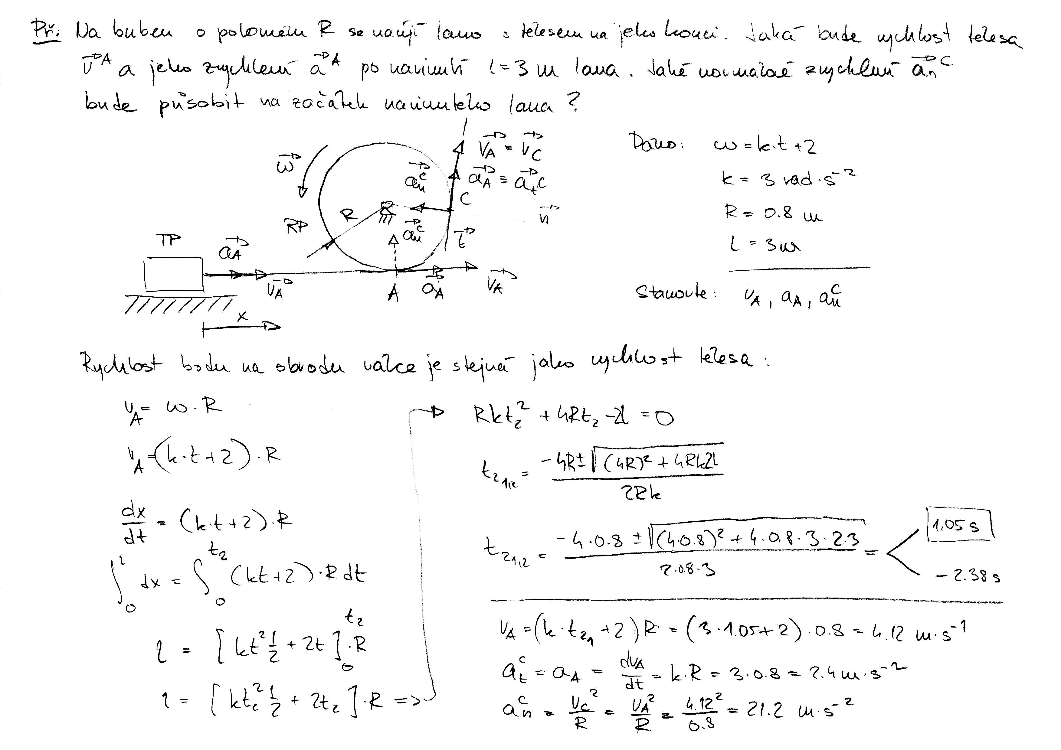
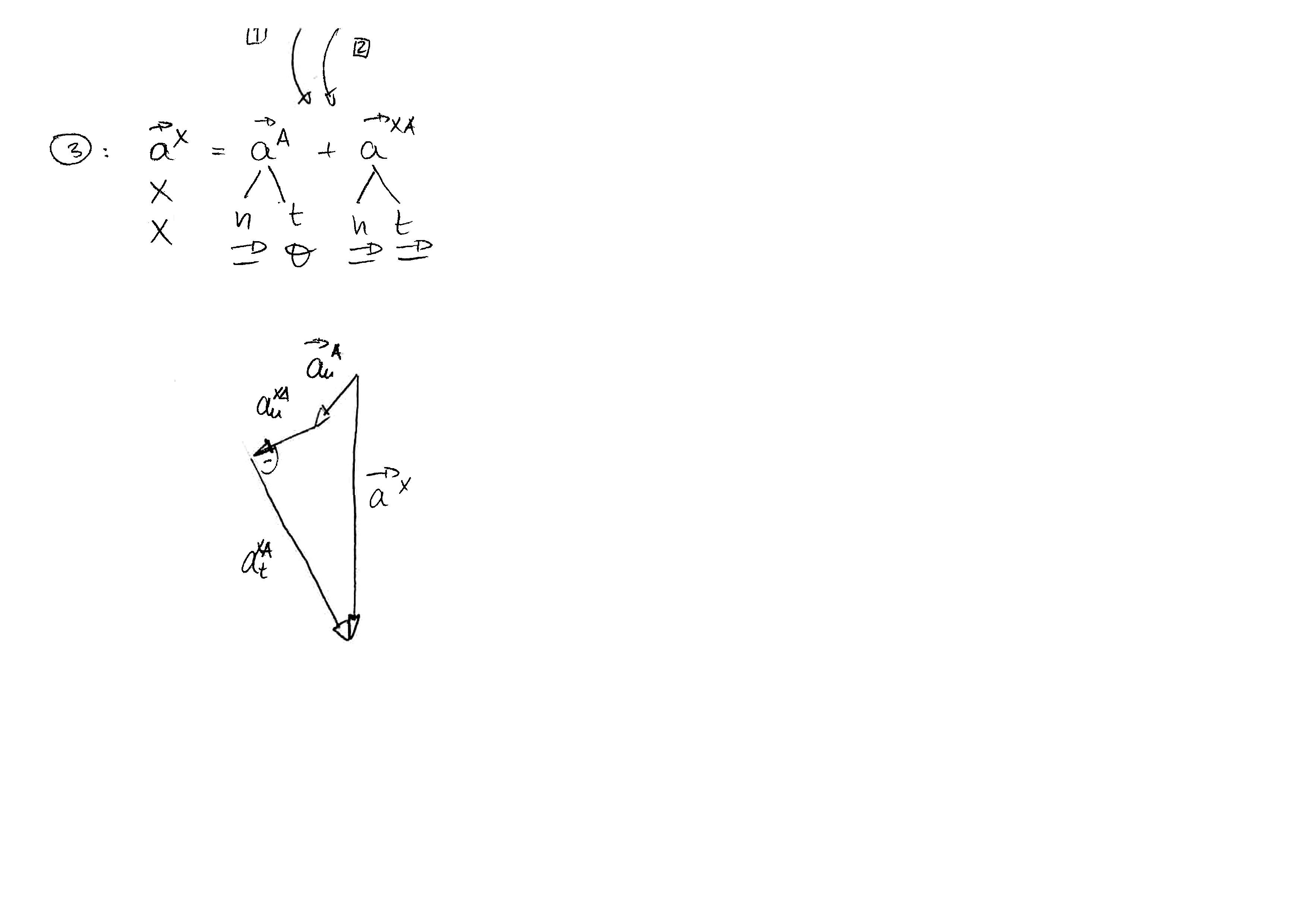
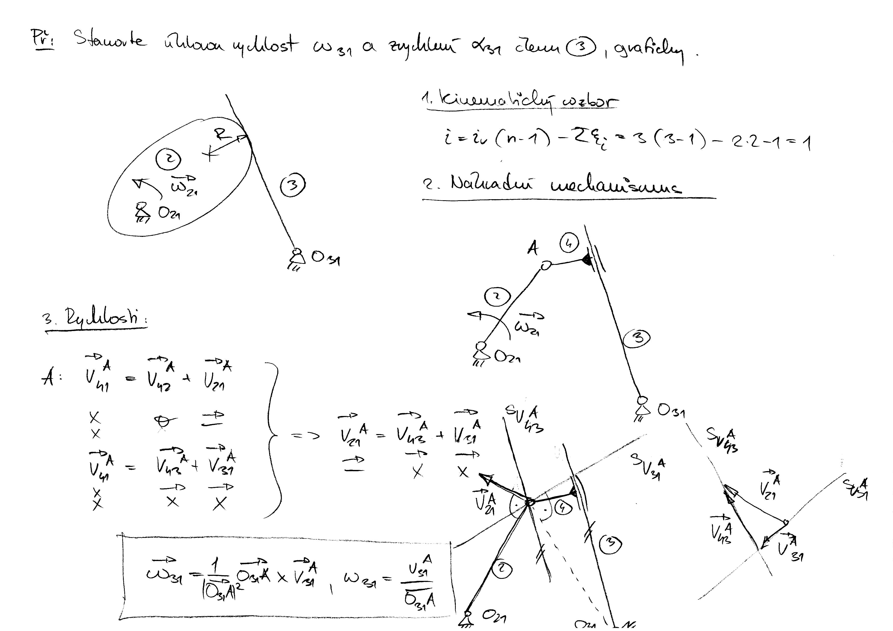
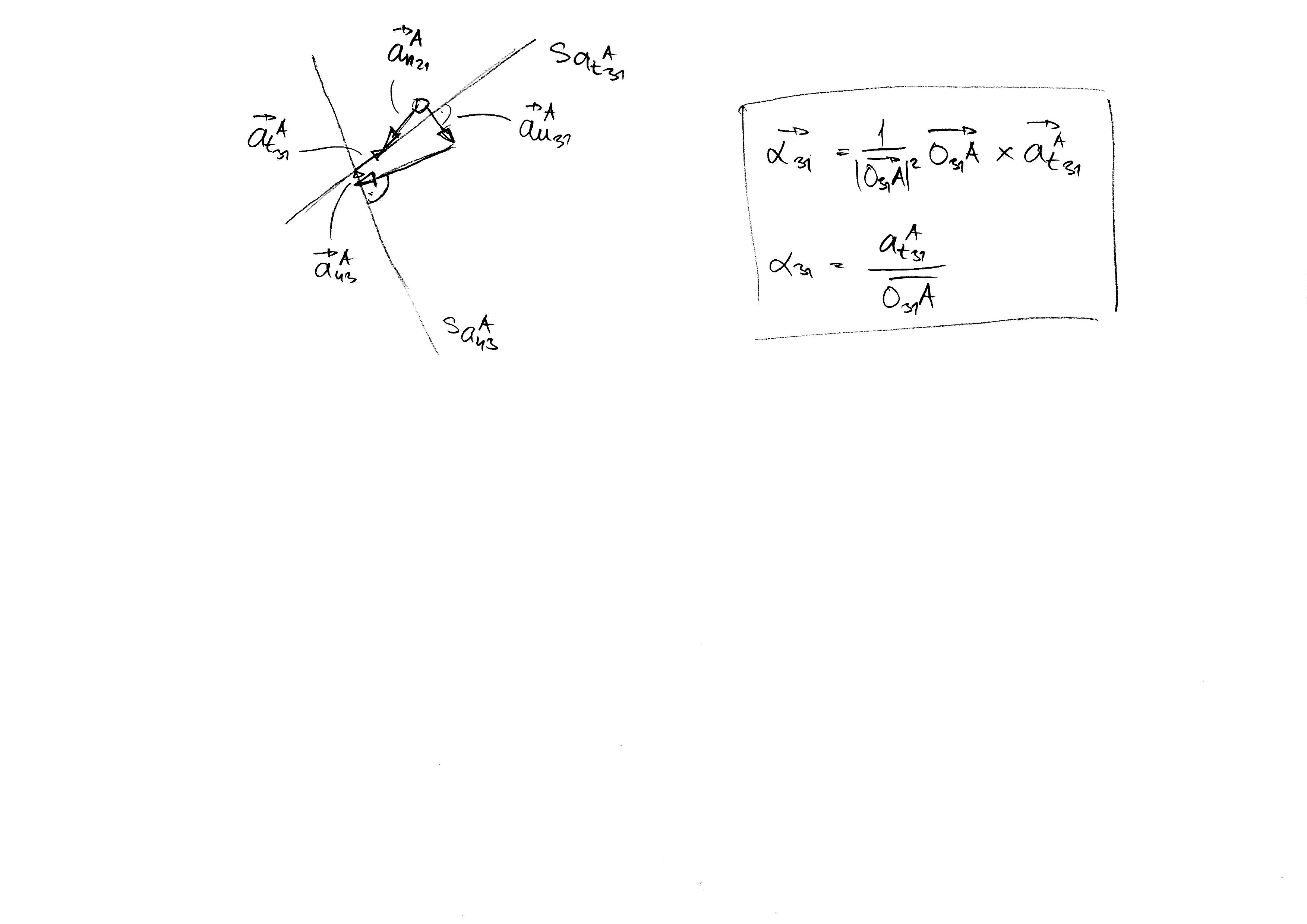
  • Cvičení 3: Rotační pohyb tělesa.

    • Ručně řešený příklad Př.1 lze stáhnout zde.

    • Ručně řešený příklad Př.2 lze stáhnout zde.

    • Ručně řešený příklad Př.3 lze stáhnout zde.

    • Ručně řešený příklad Př.4 lze stáhnout zde a zde.

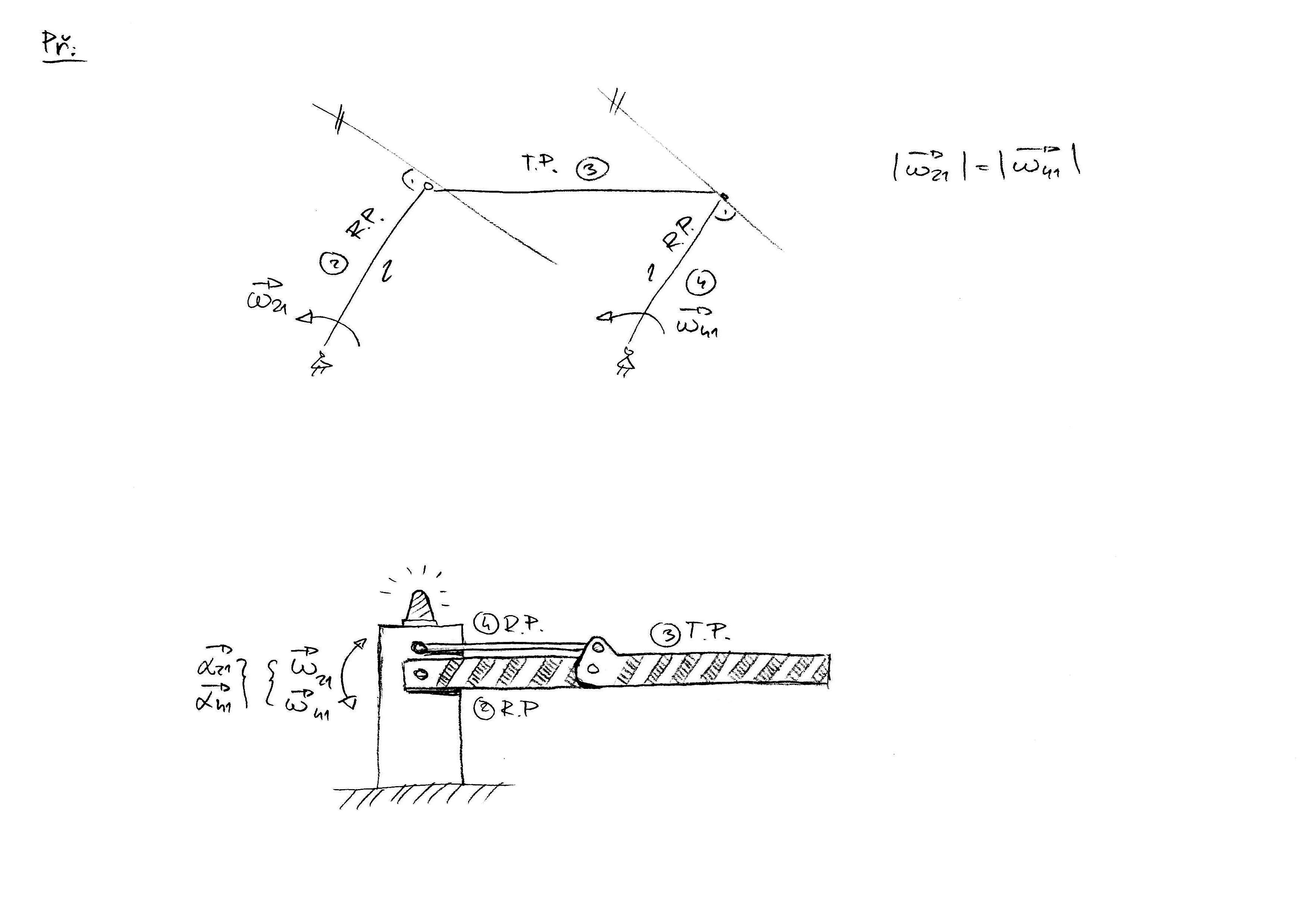
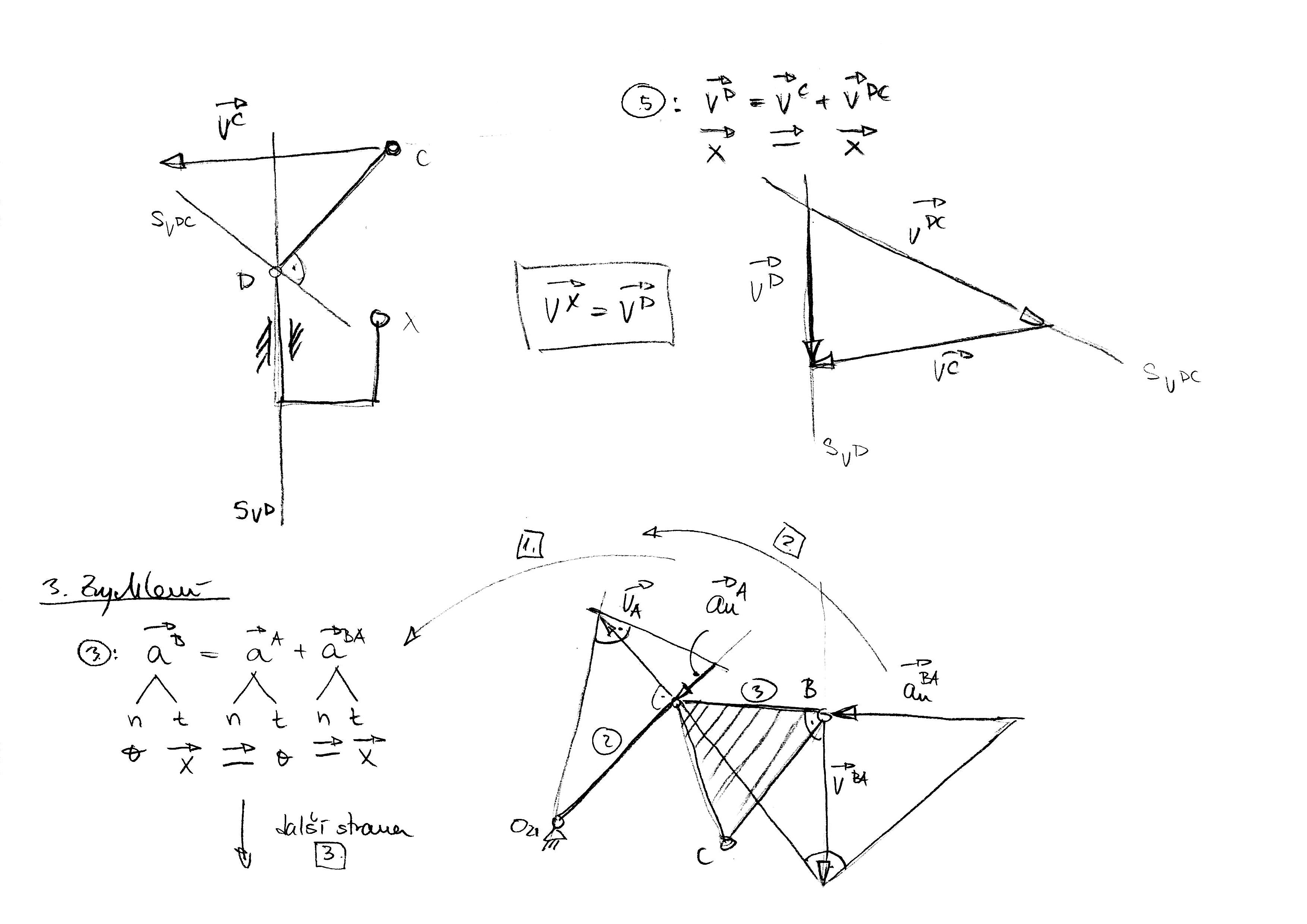
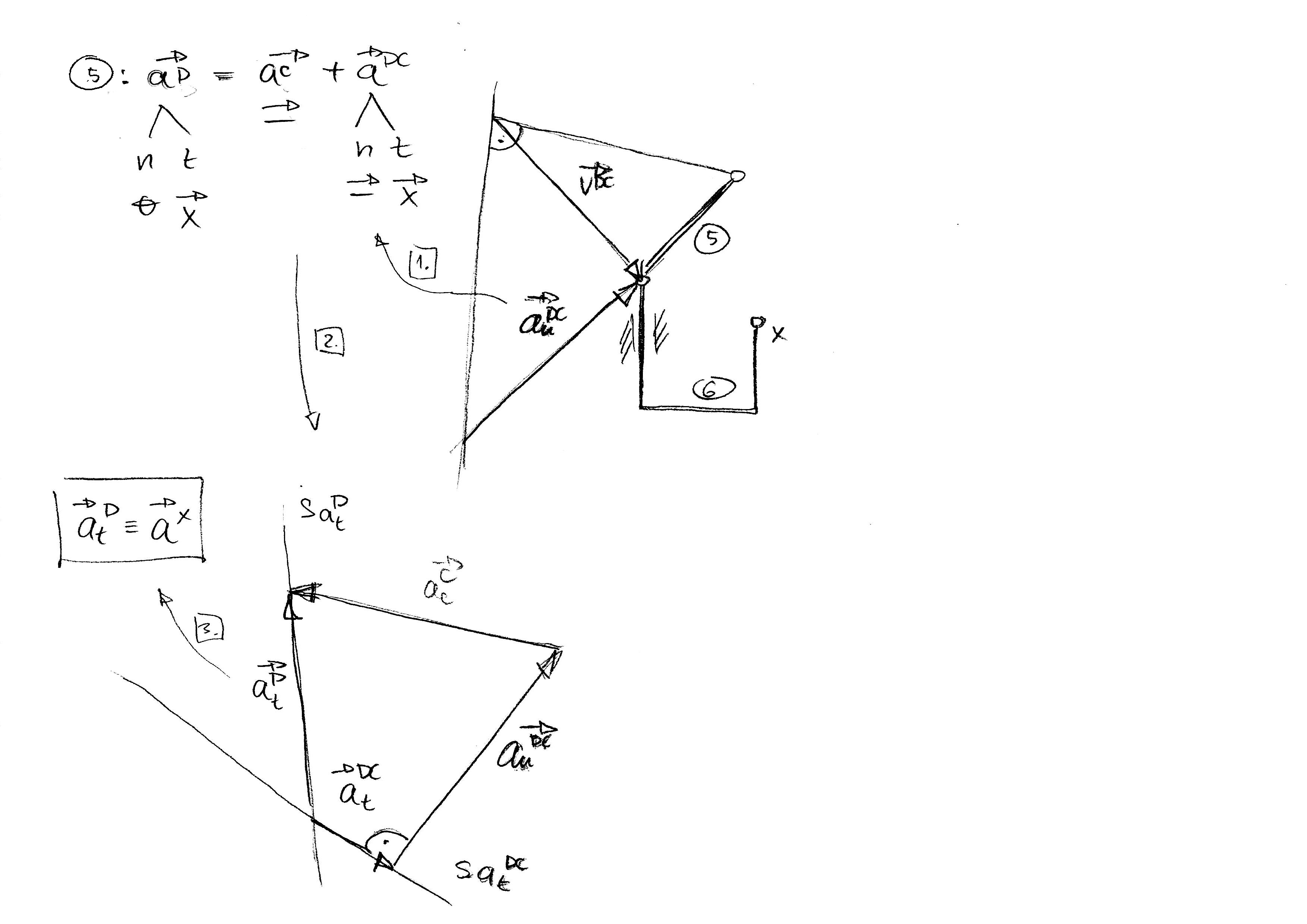
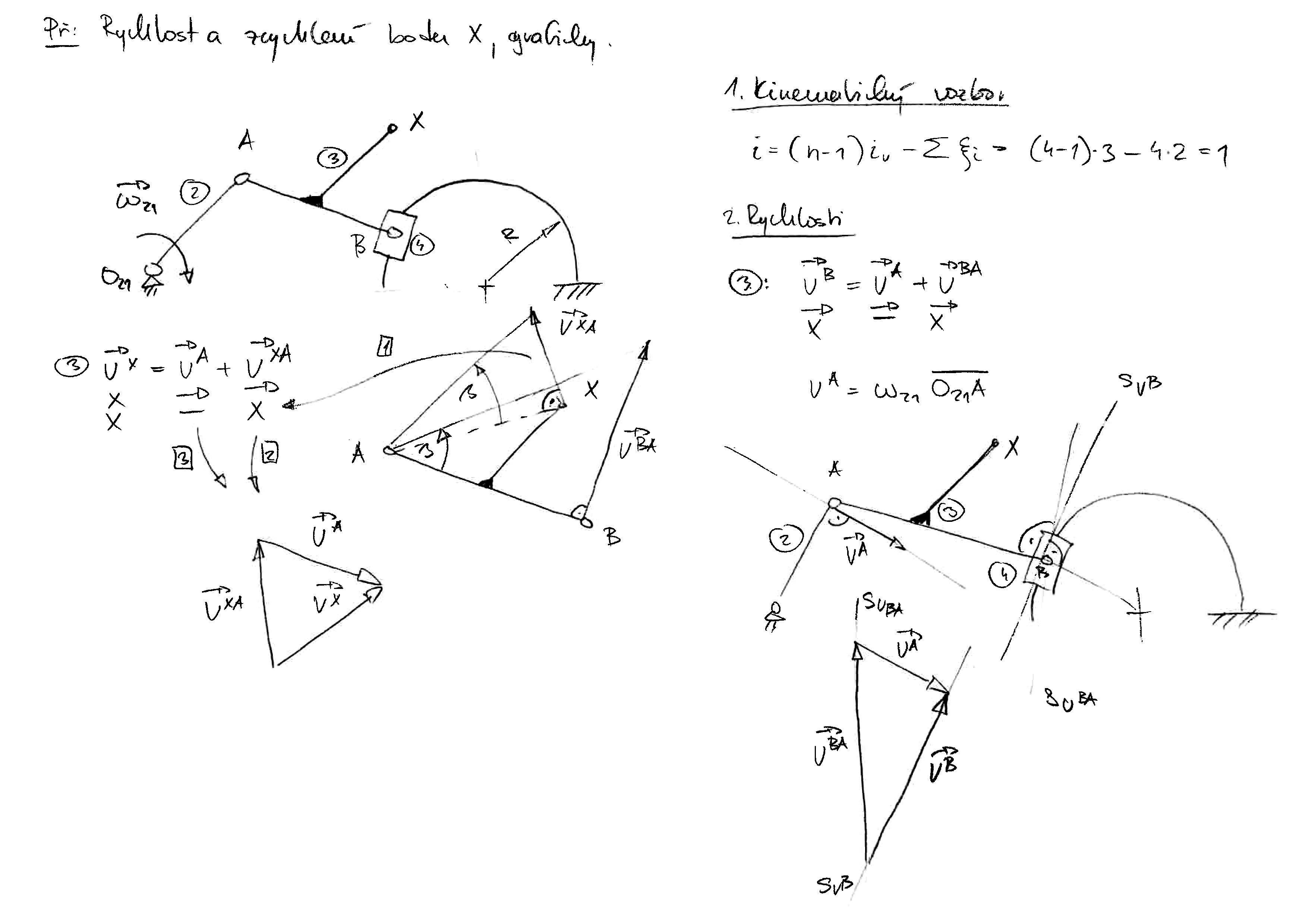
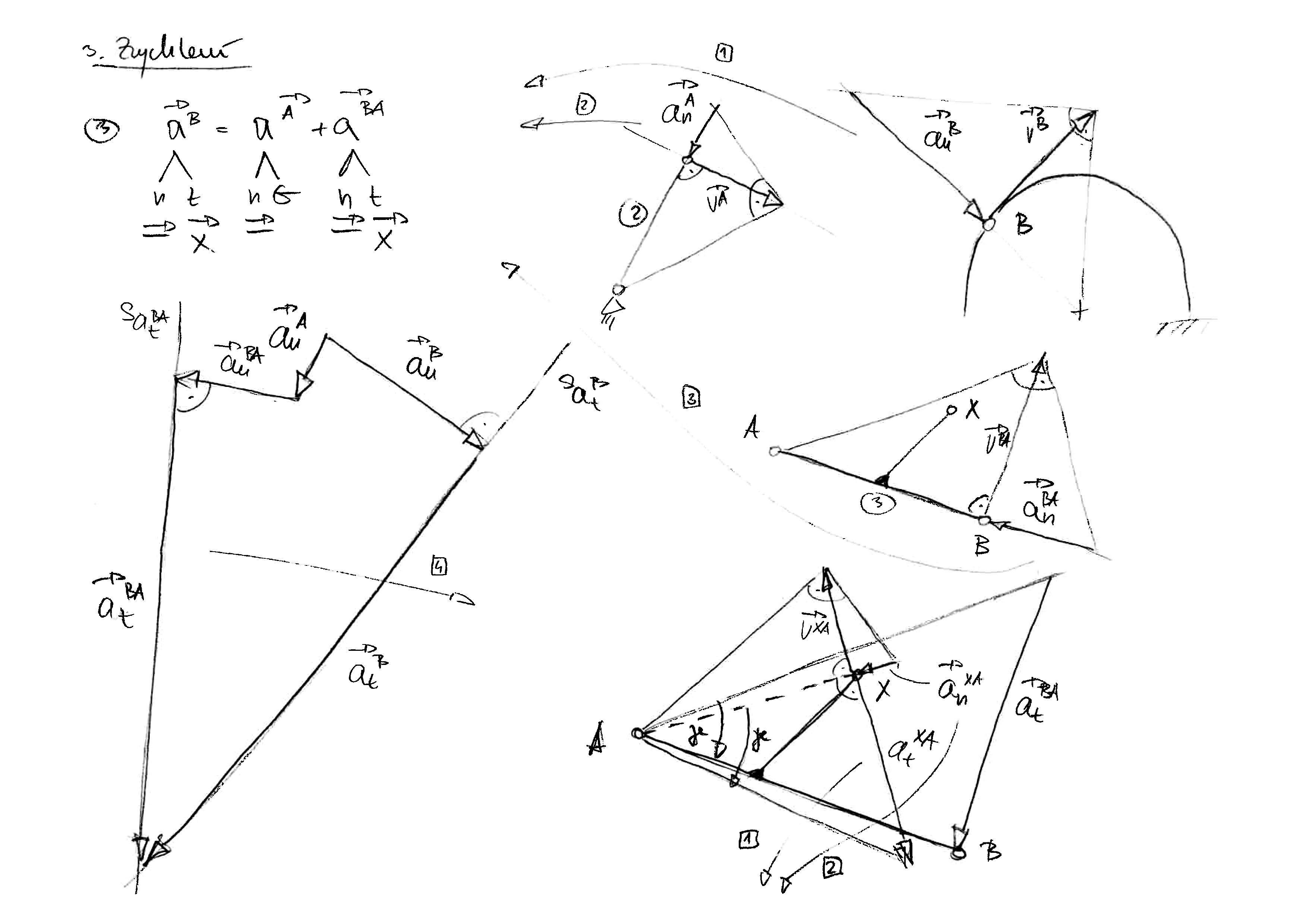
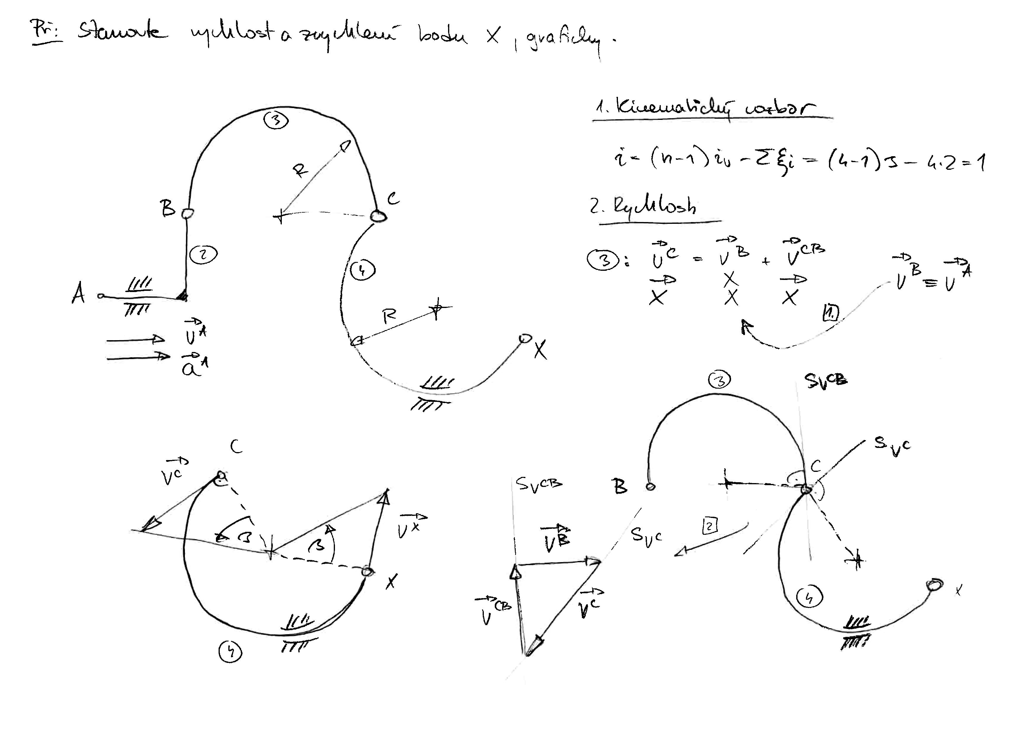
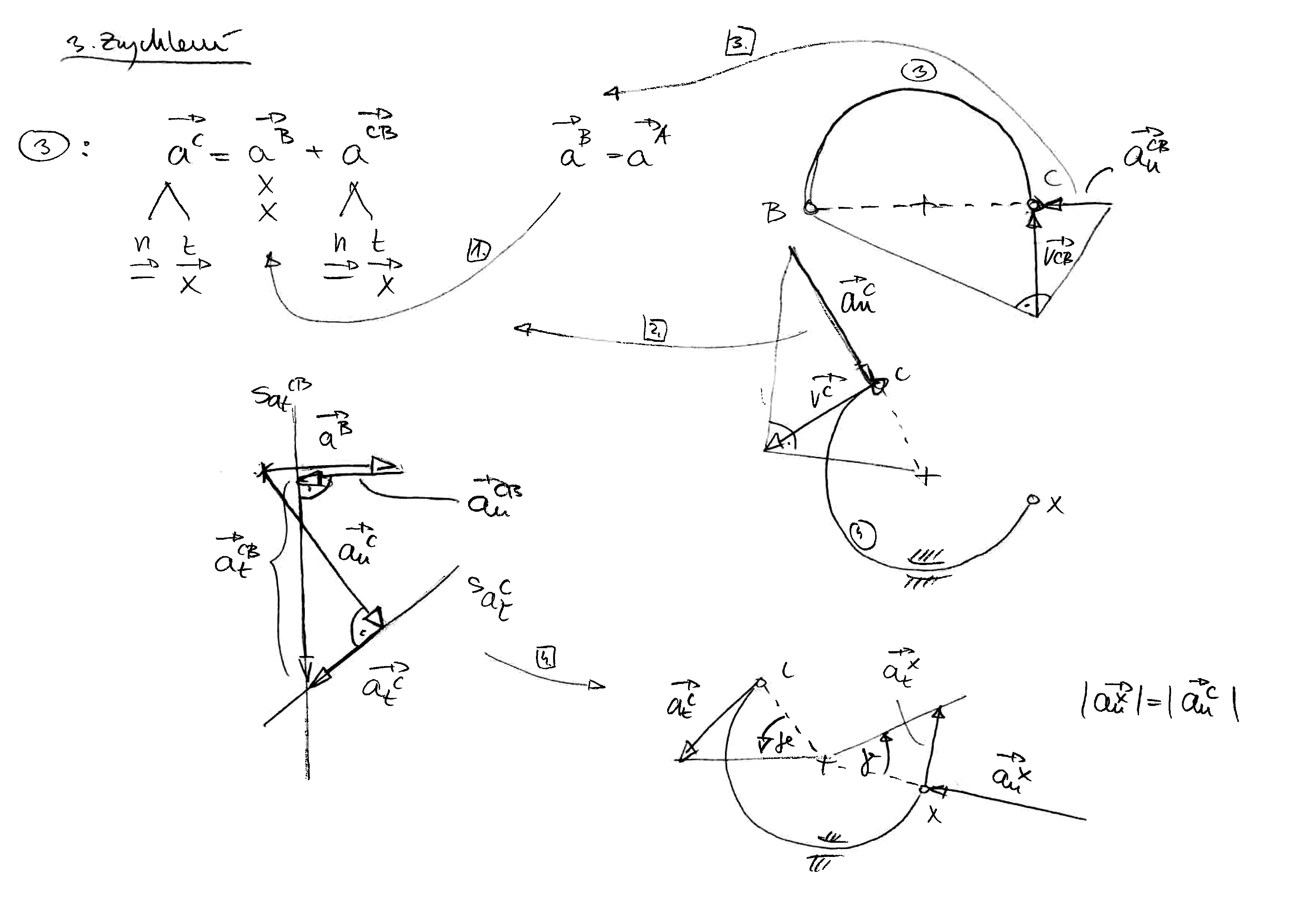
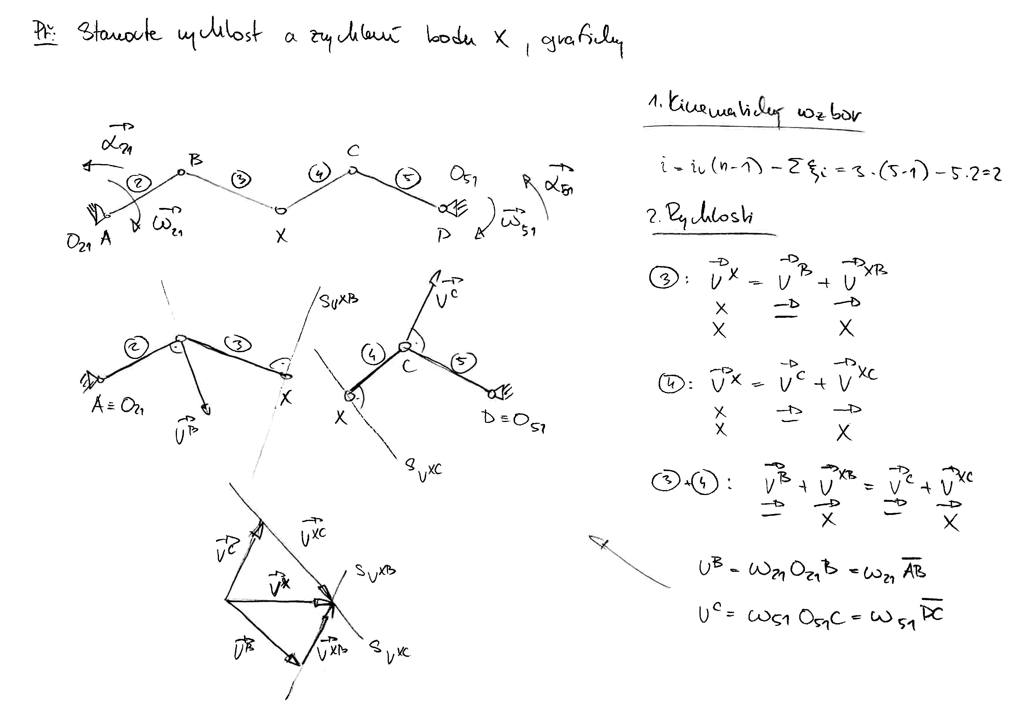
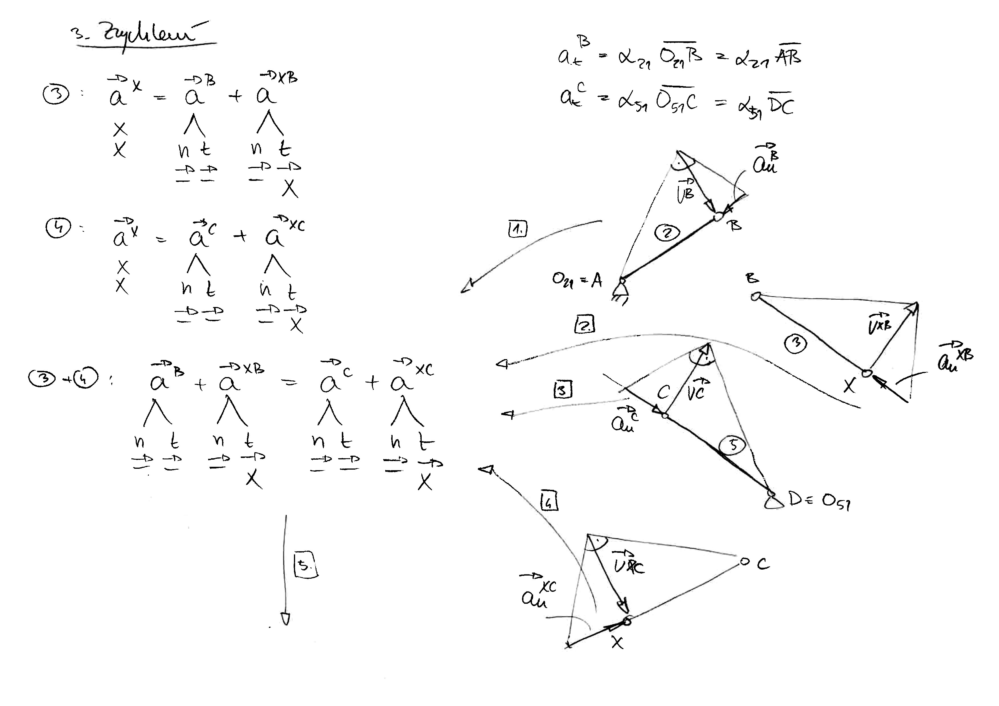
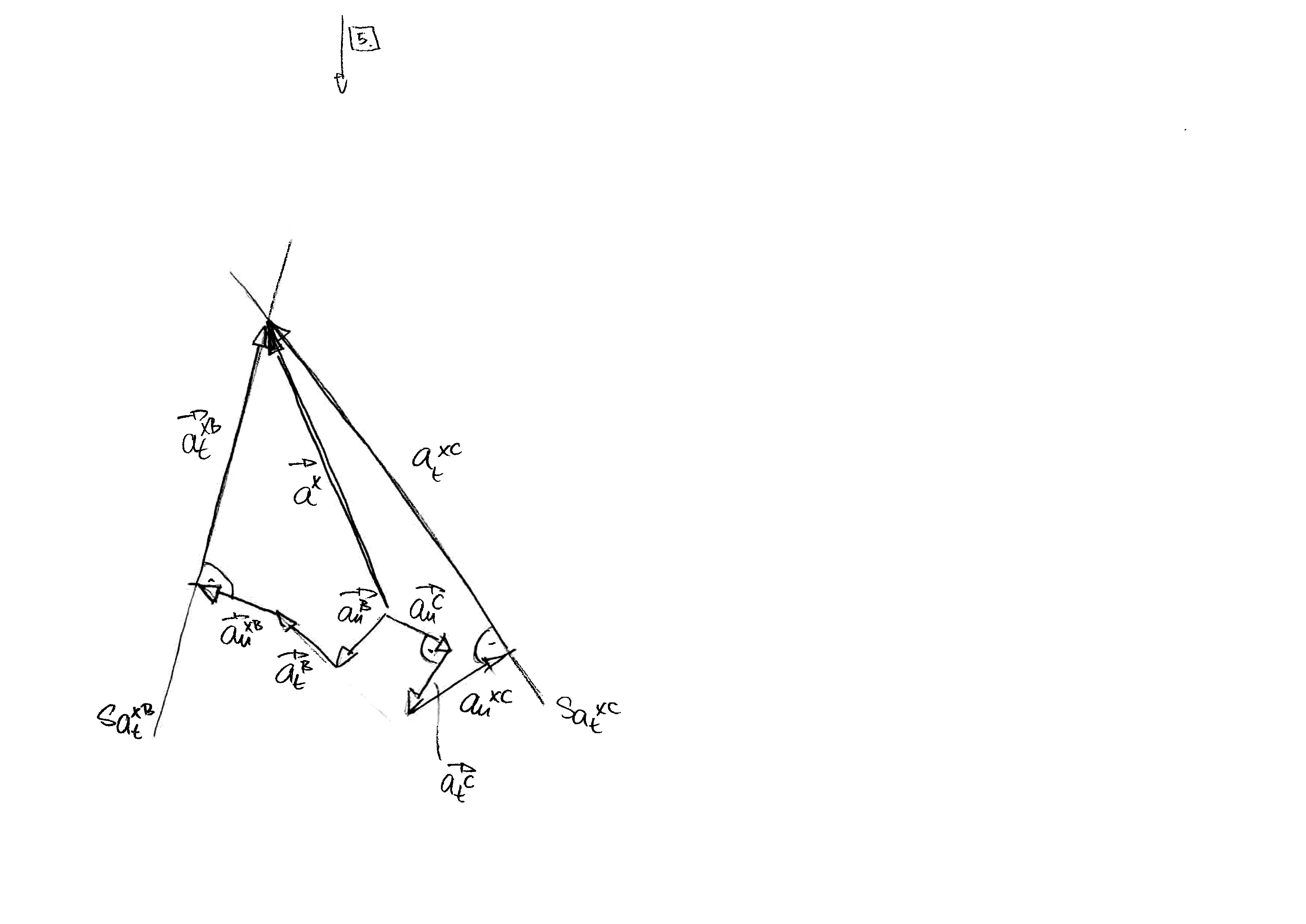
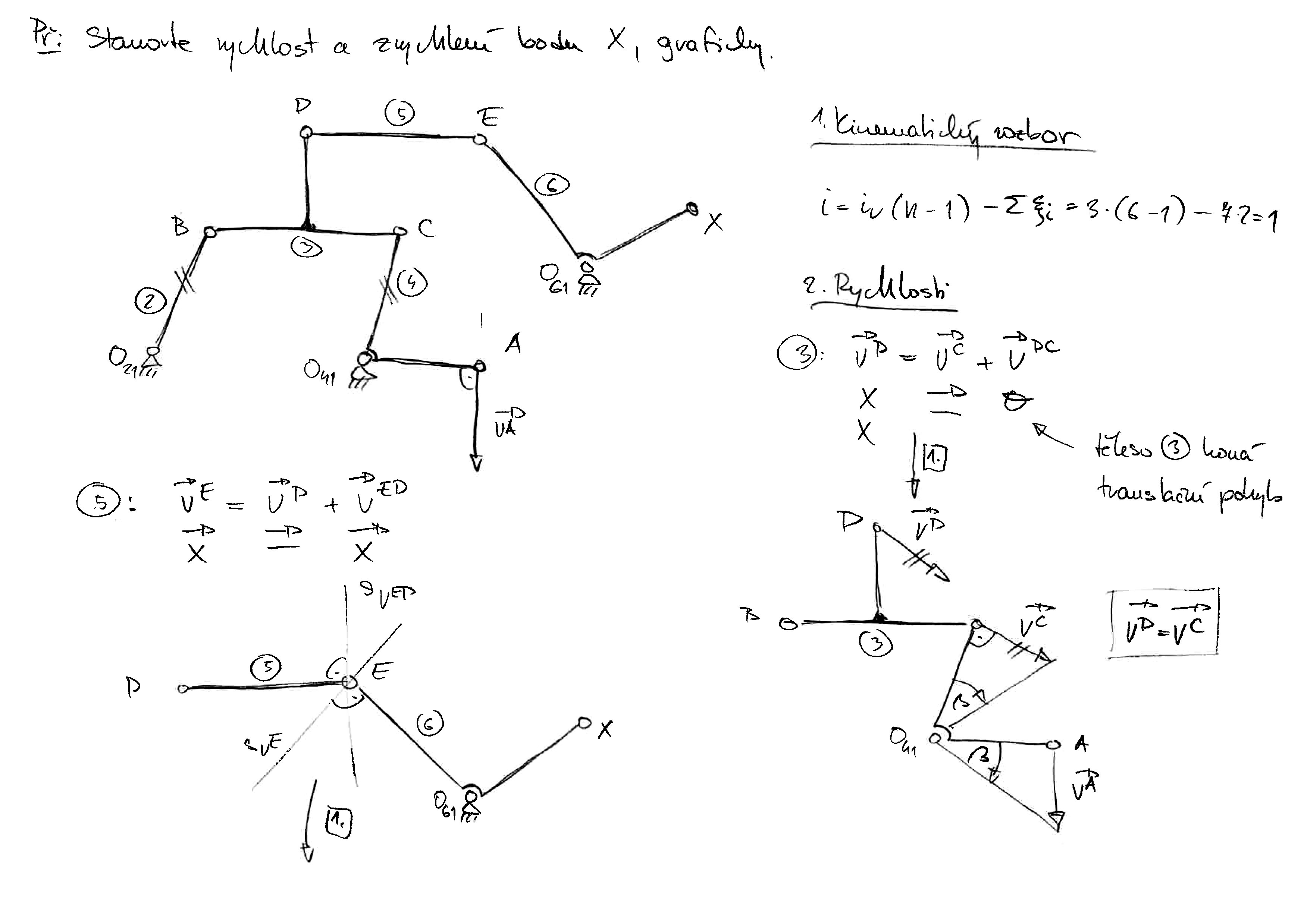
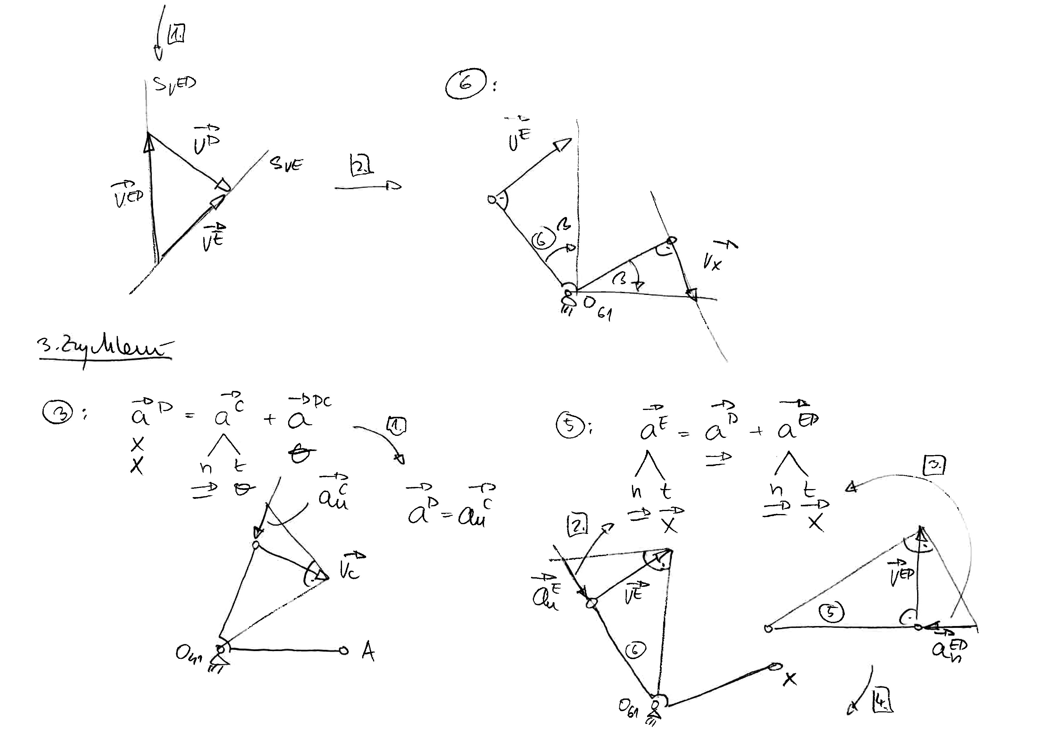
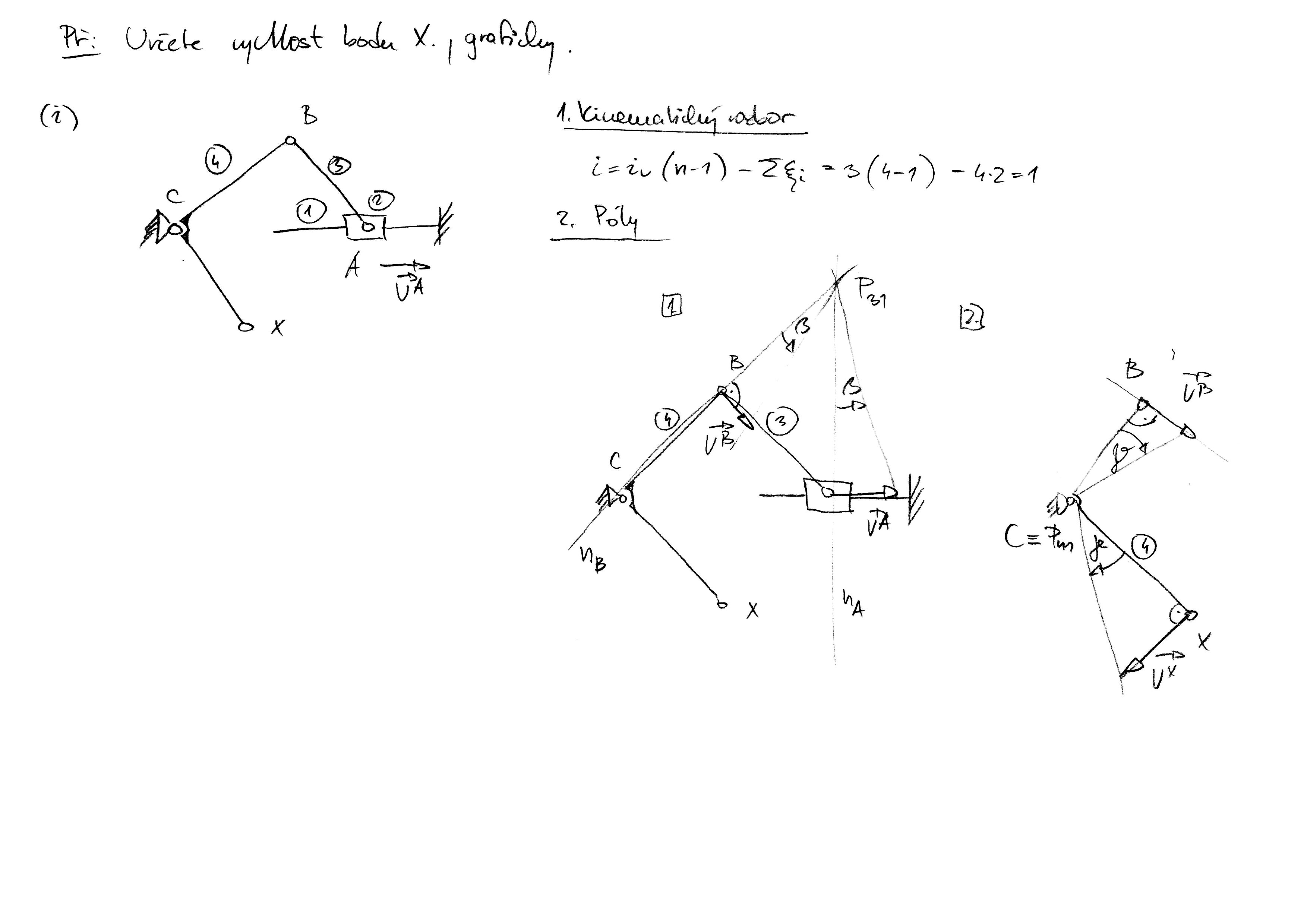
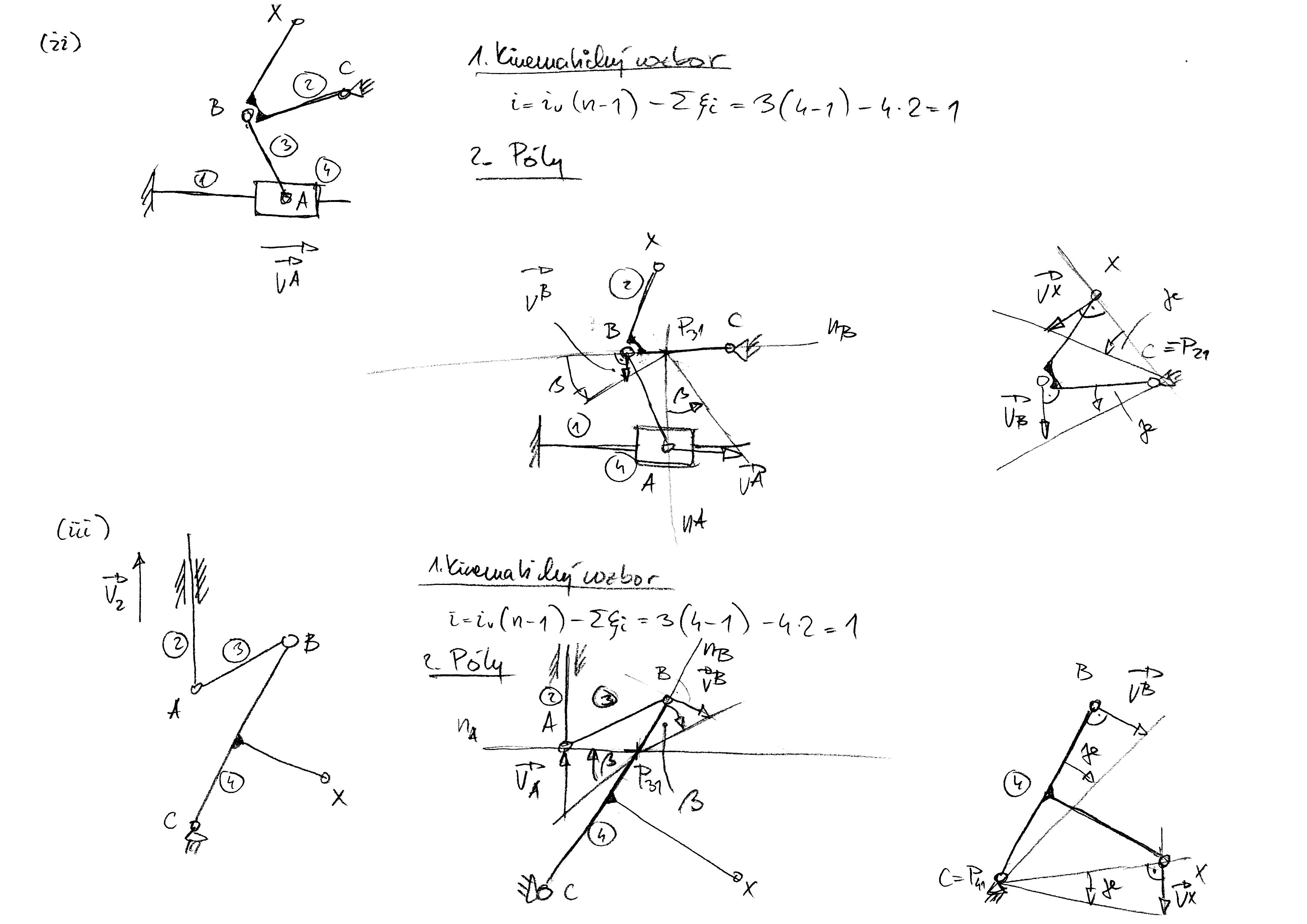
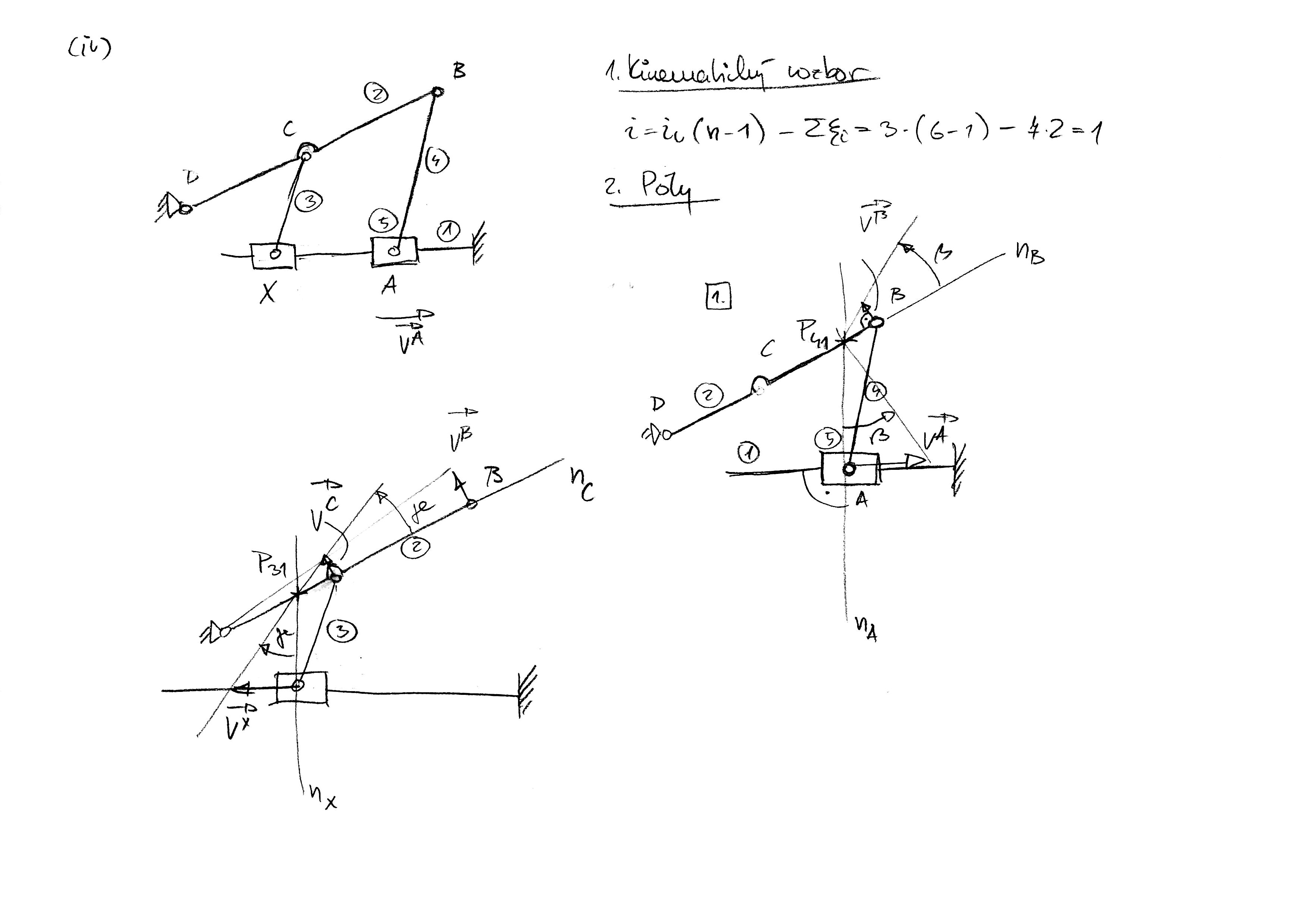
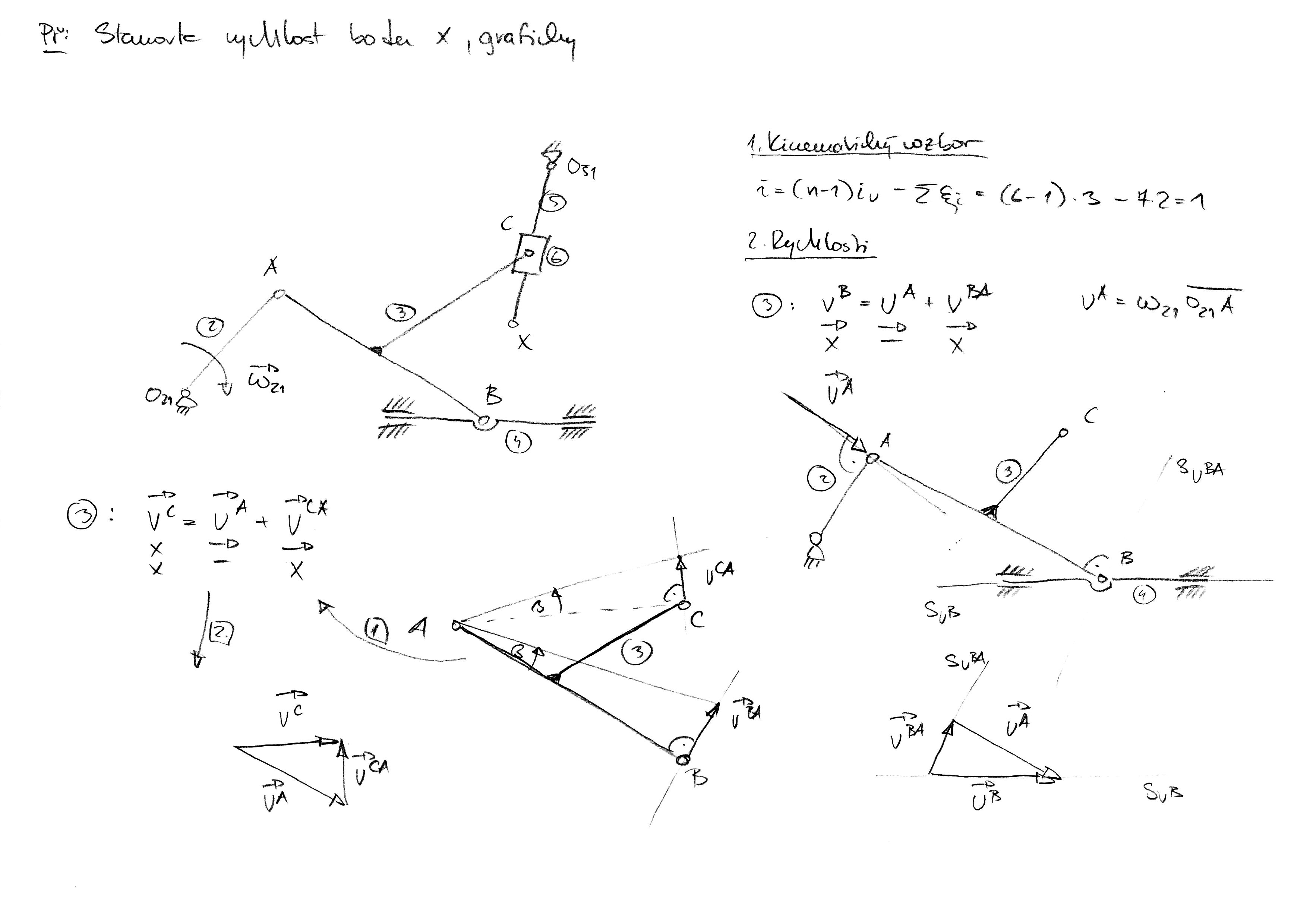
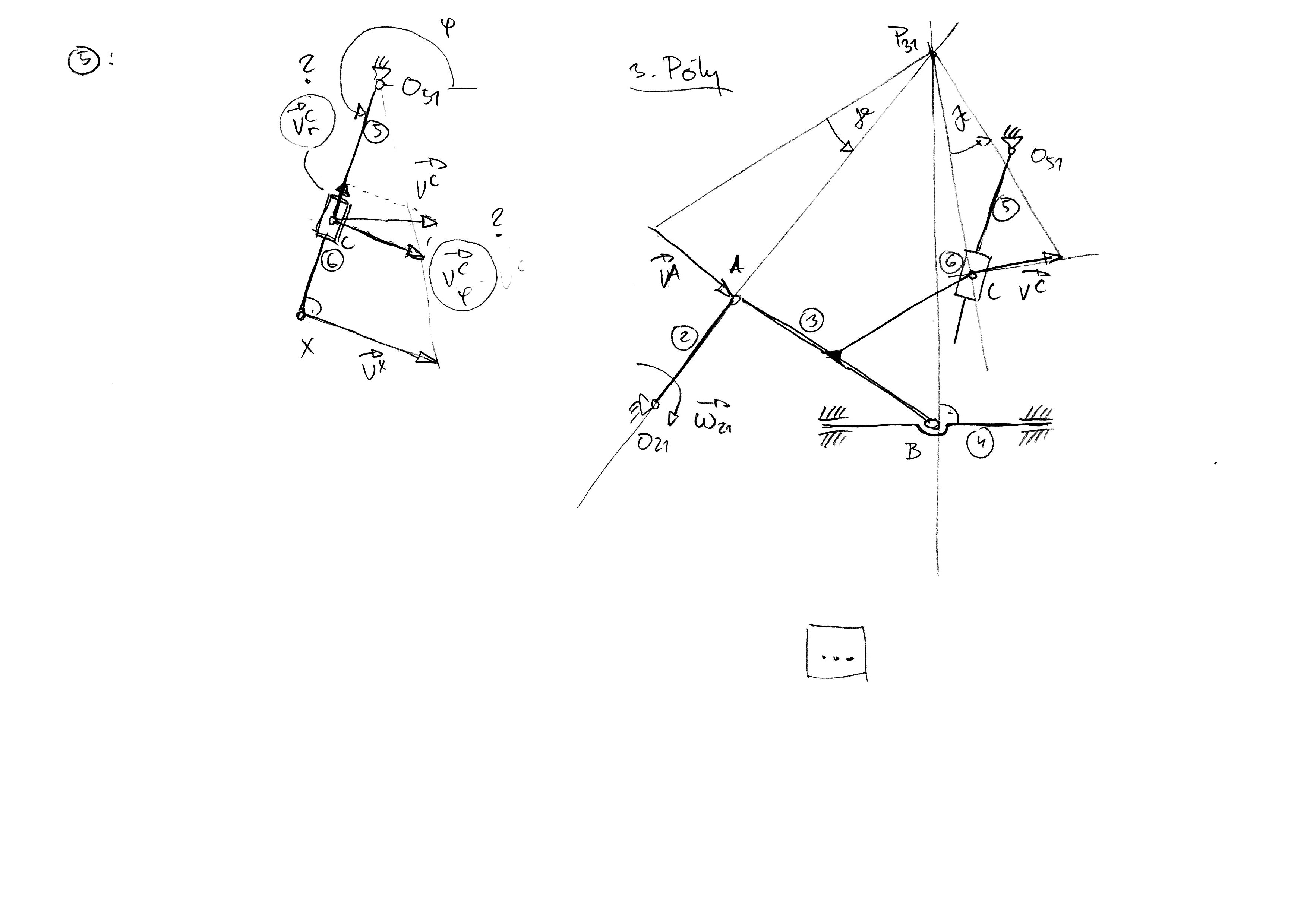
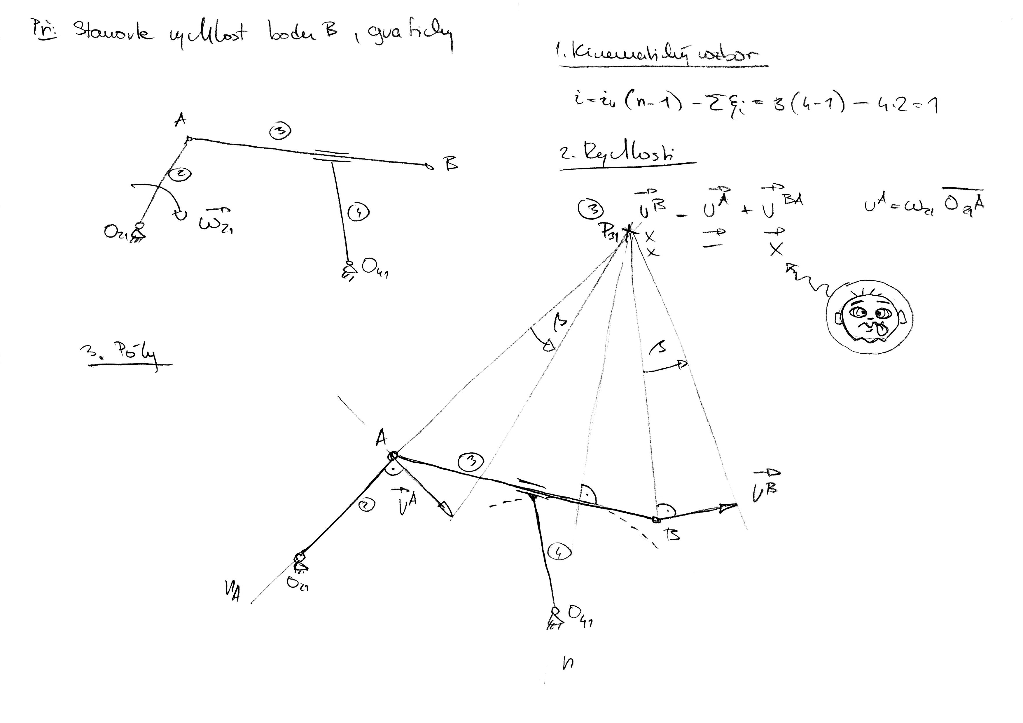
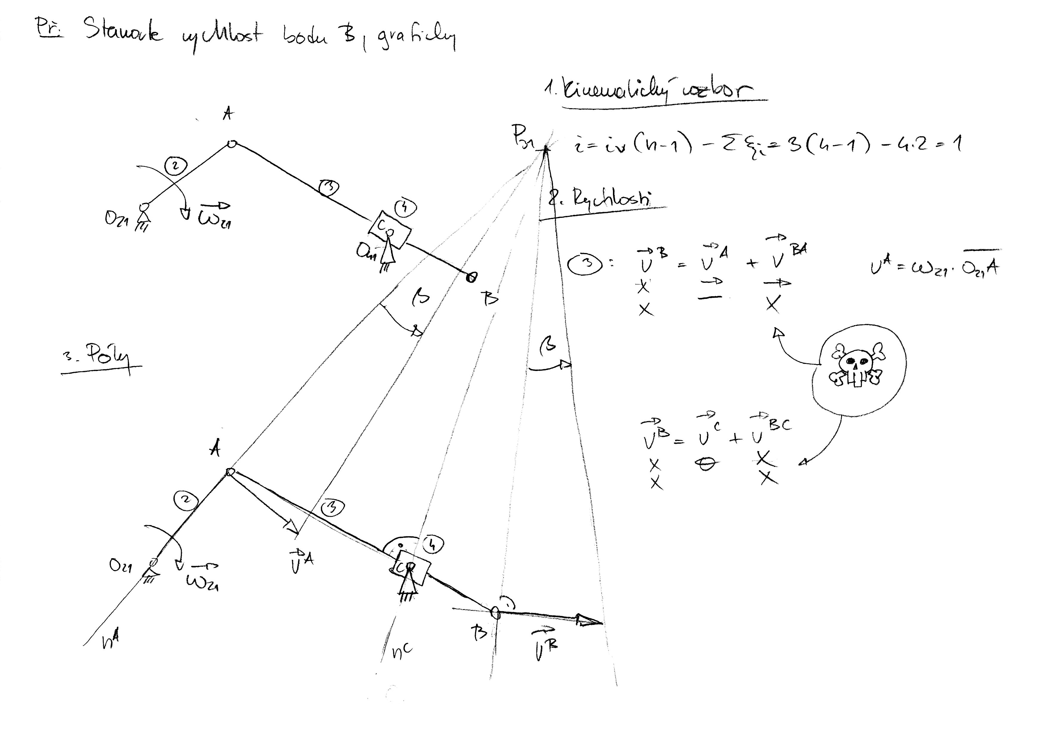
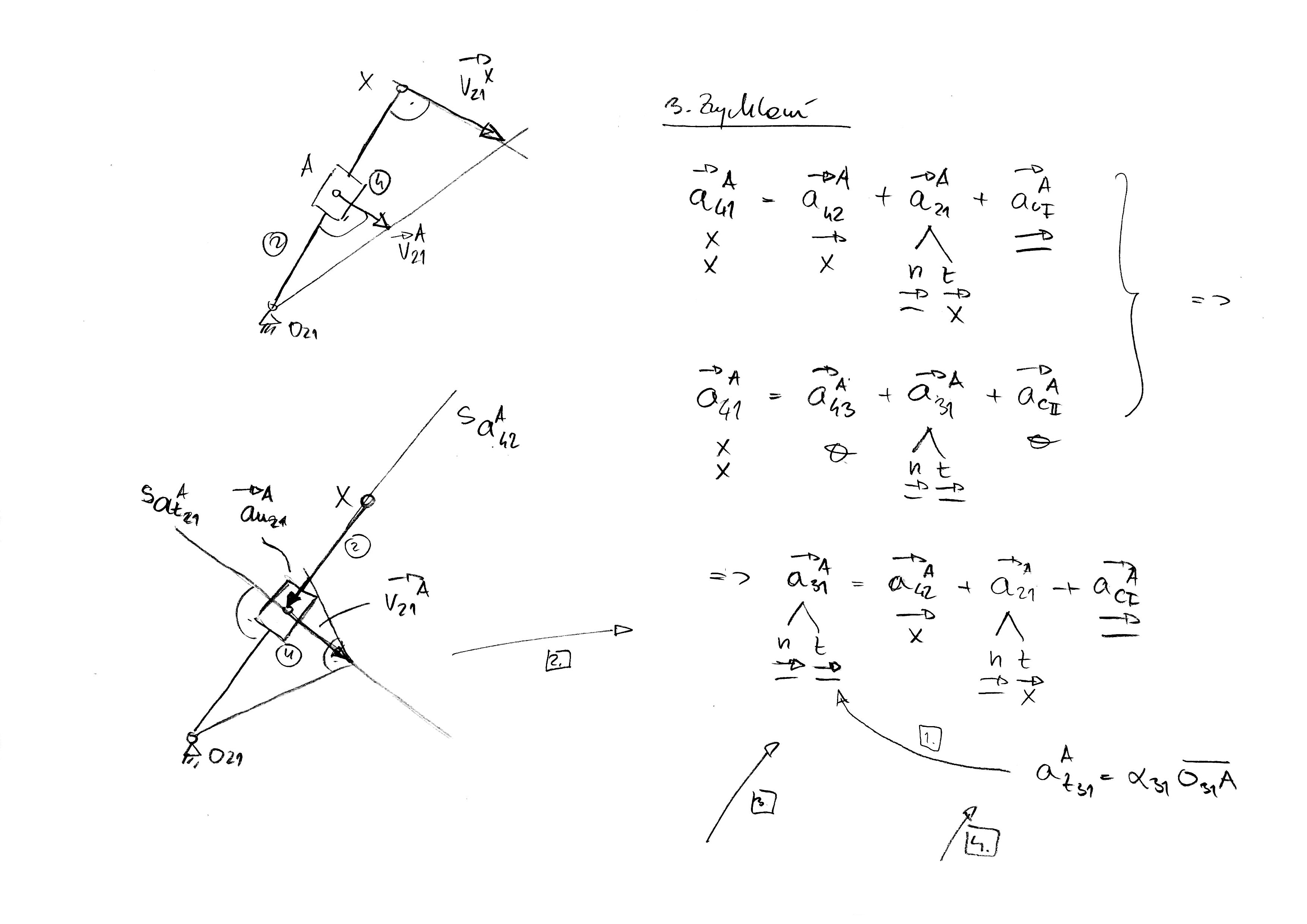
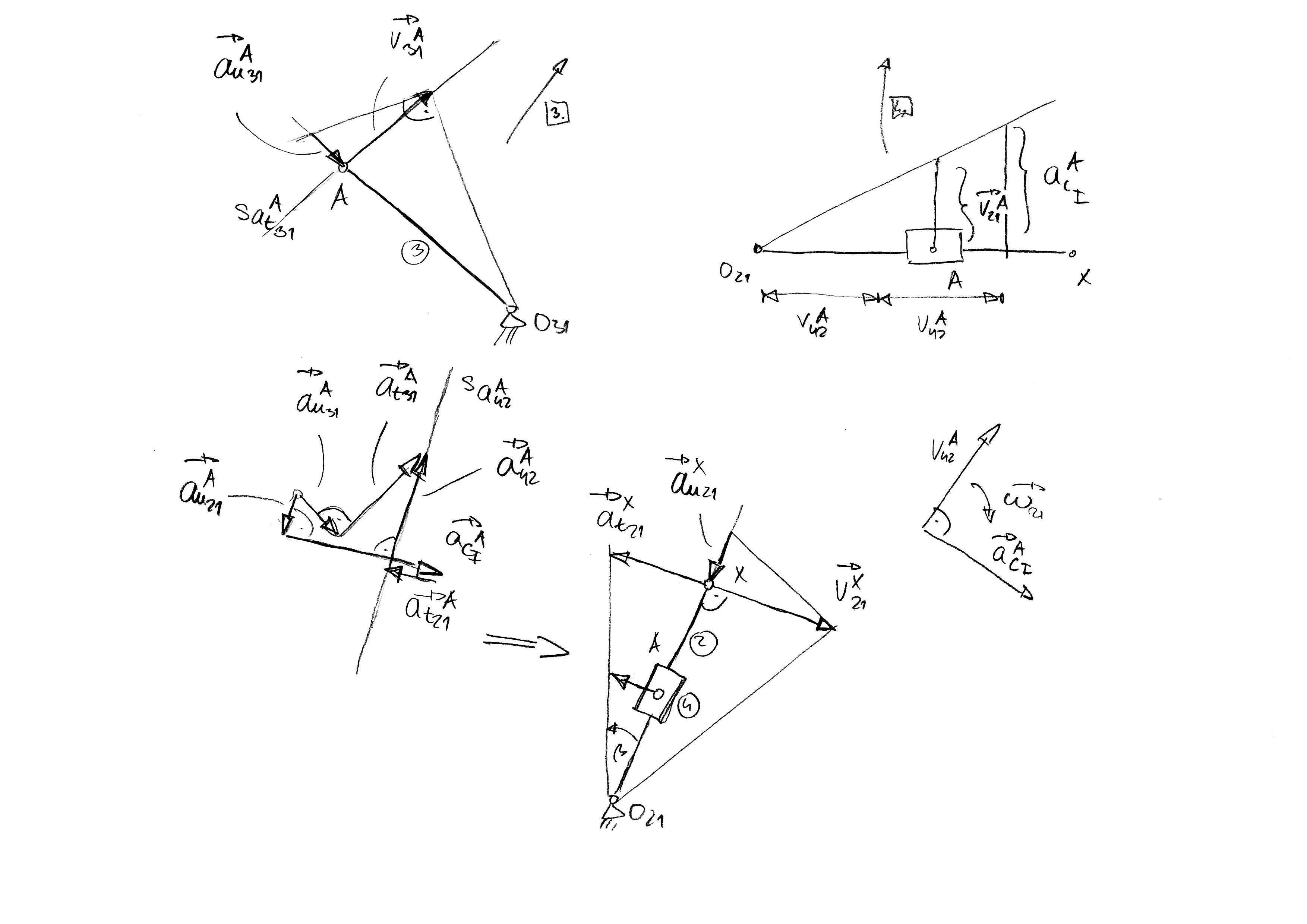
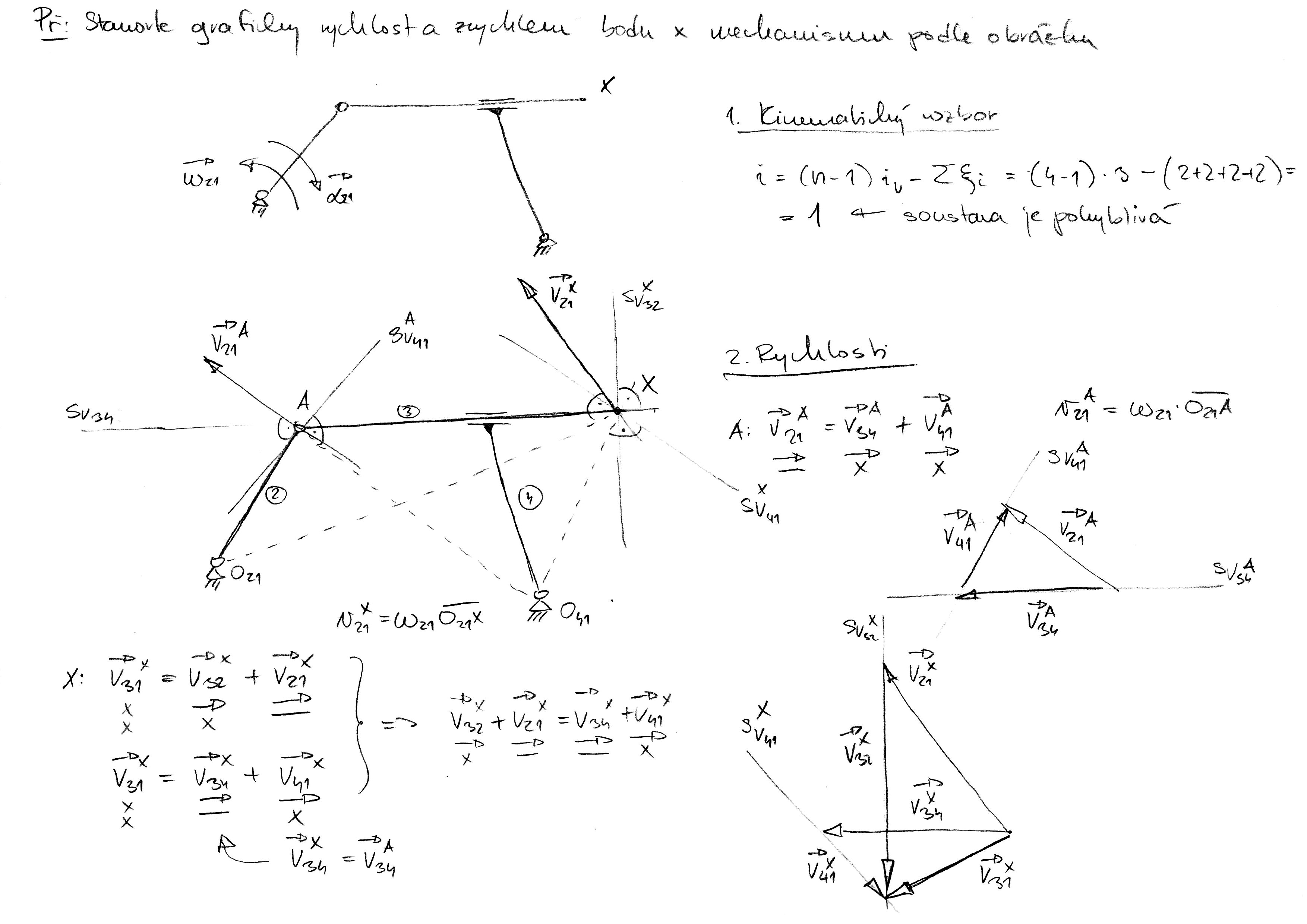
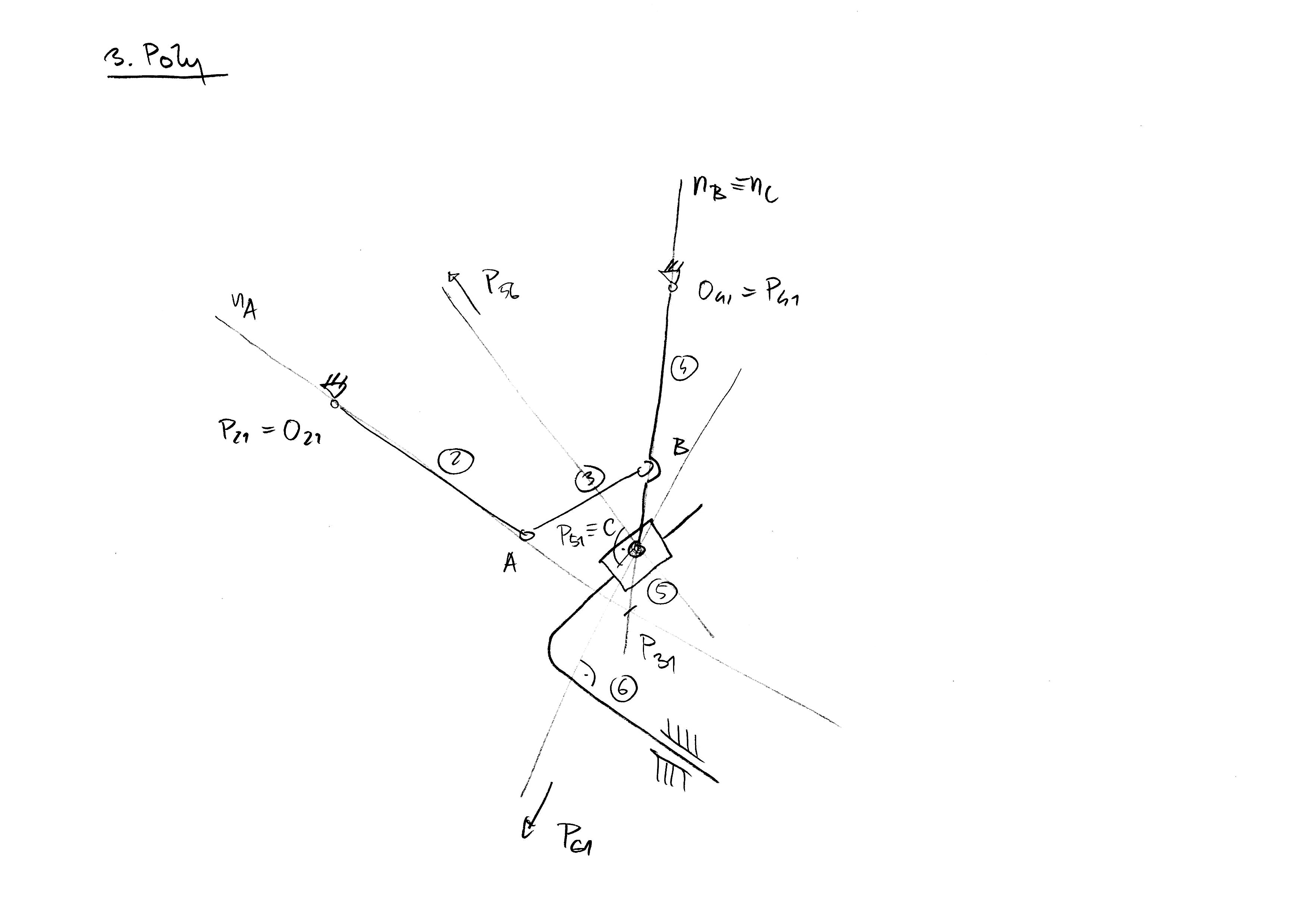
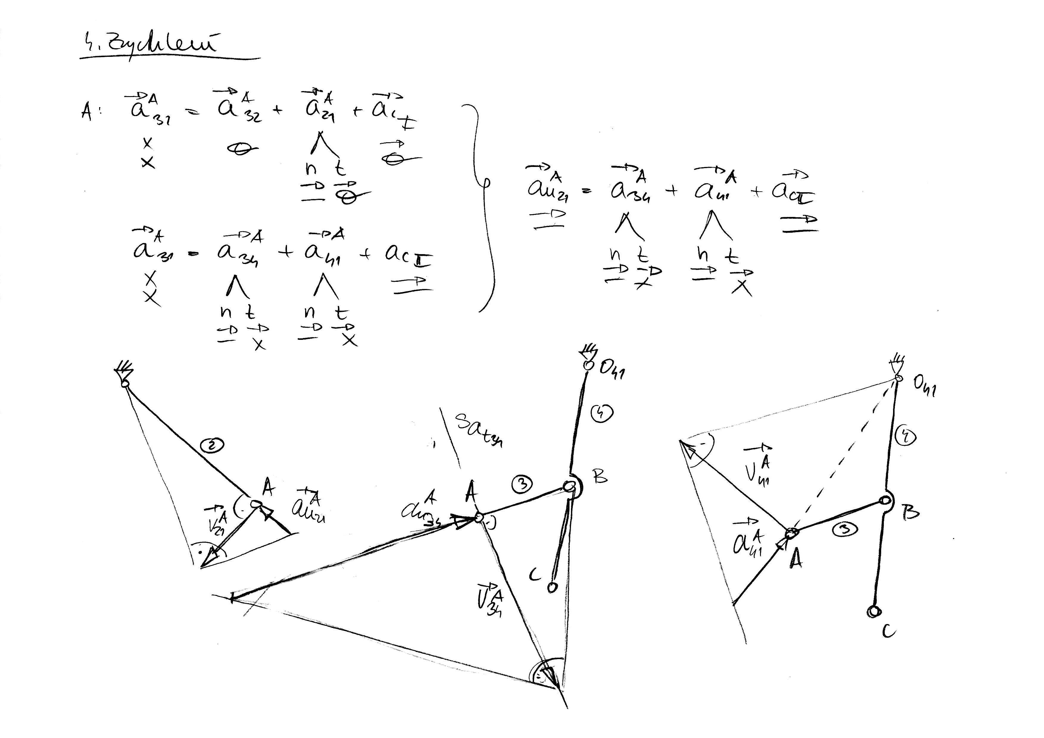
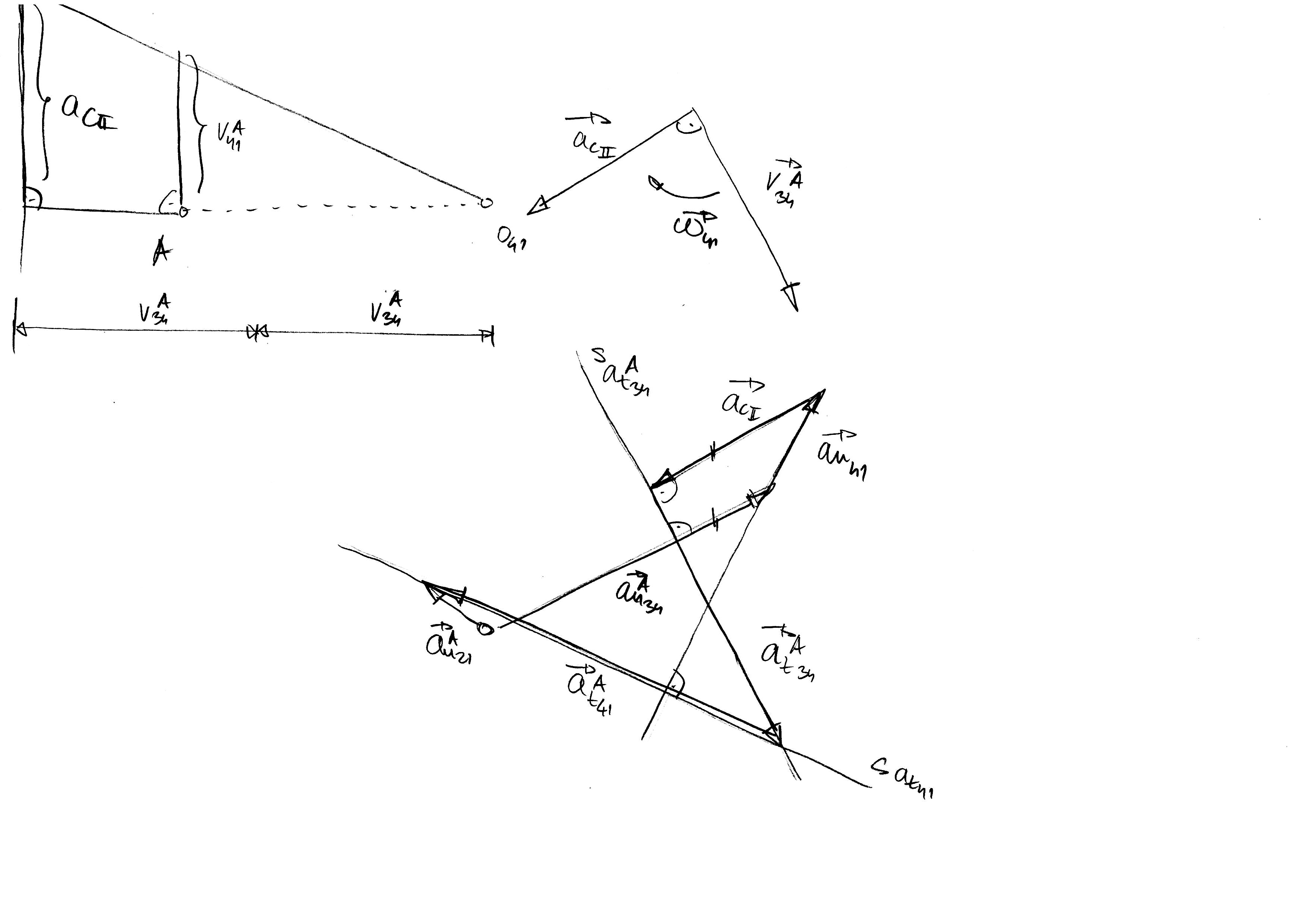
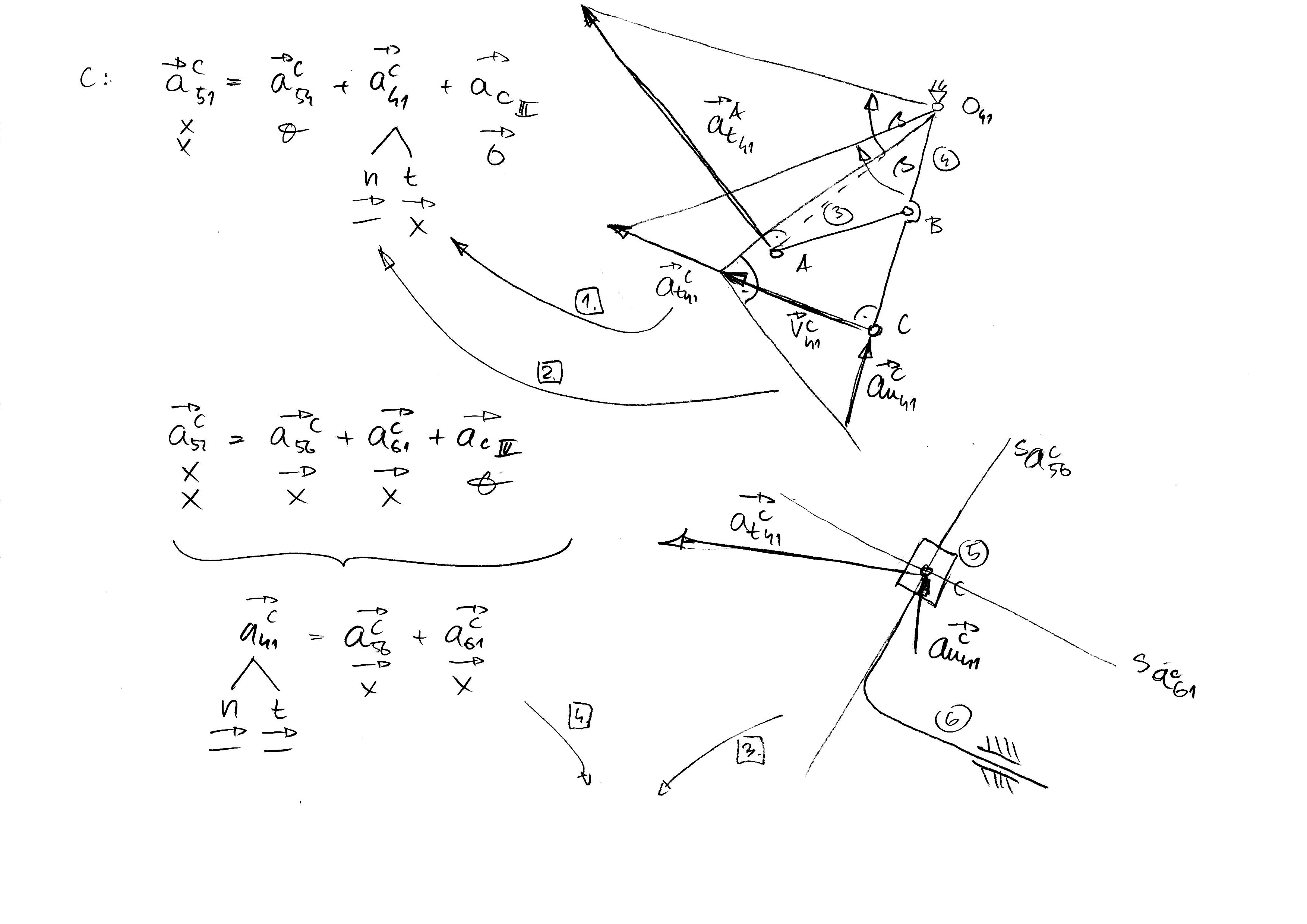
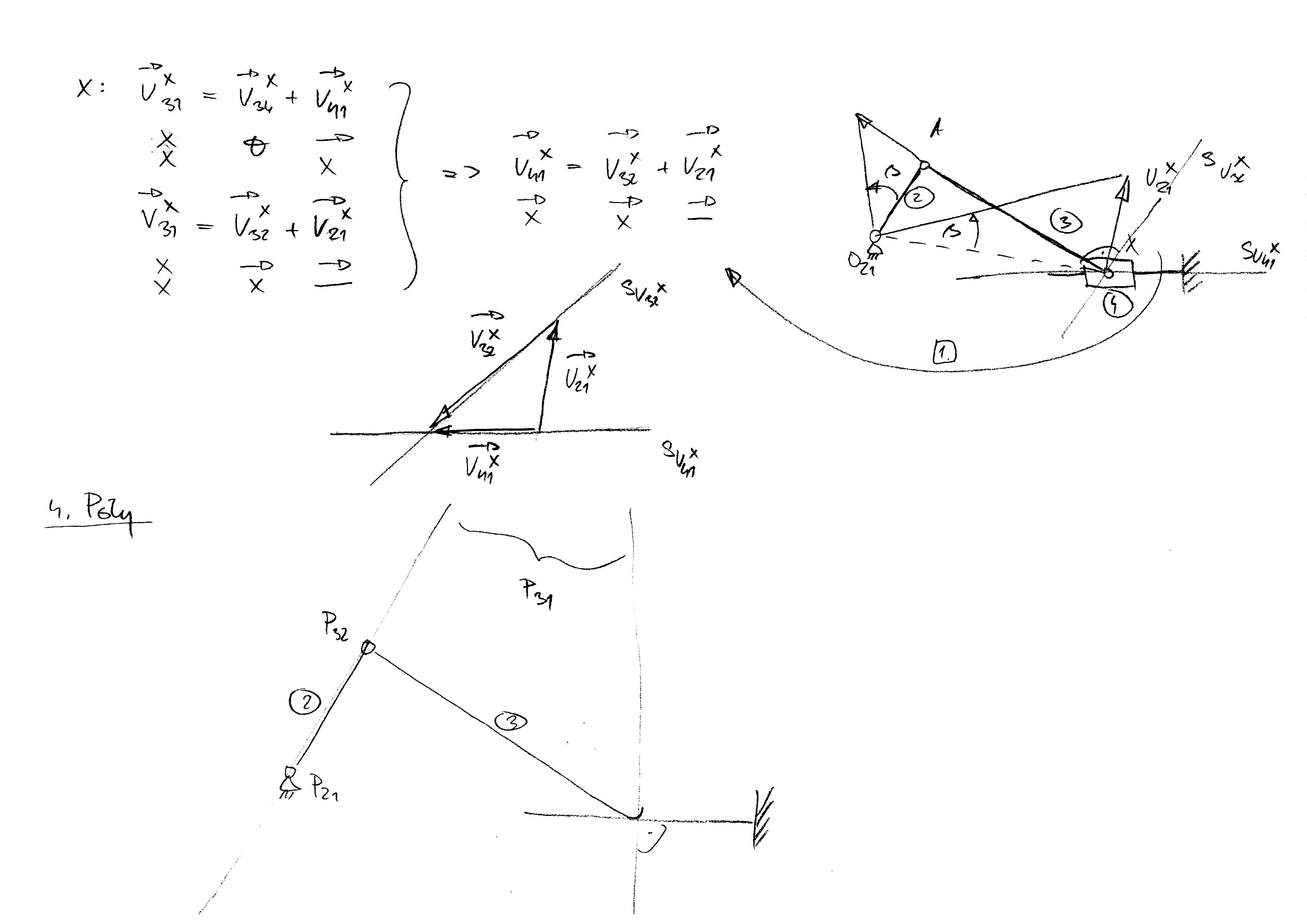
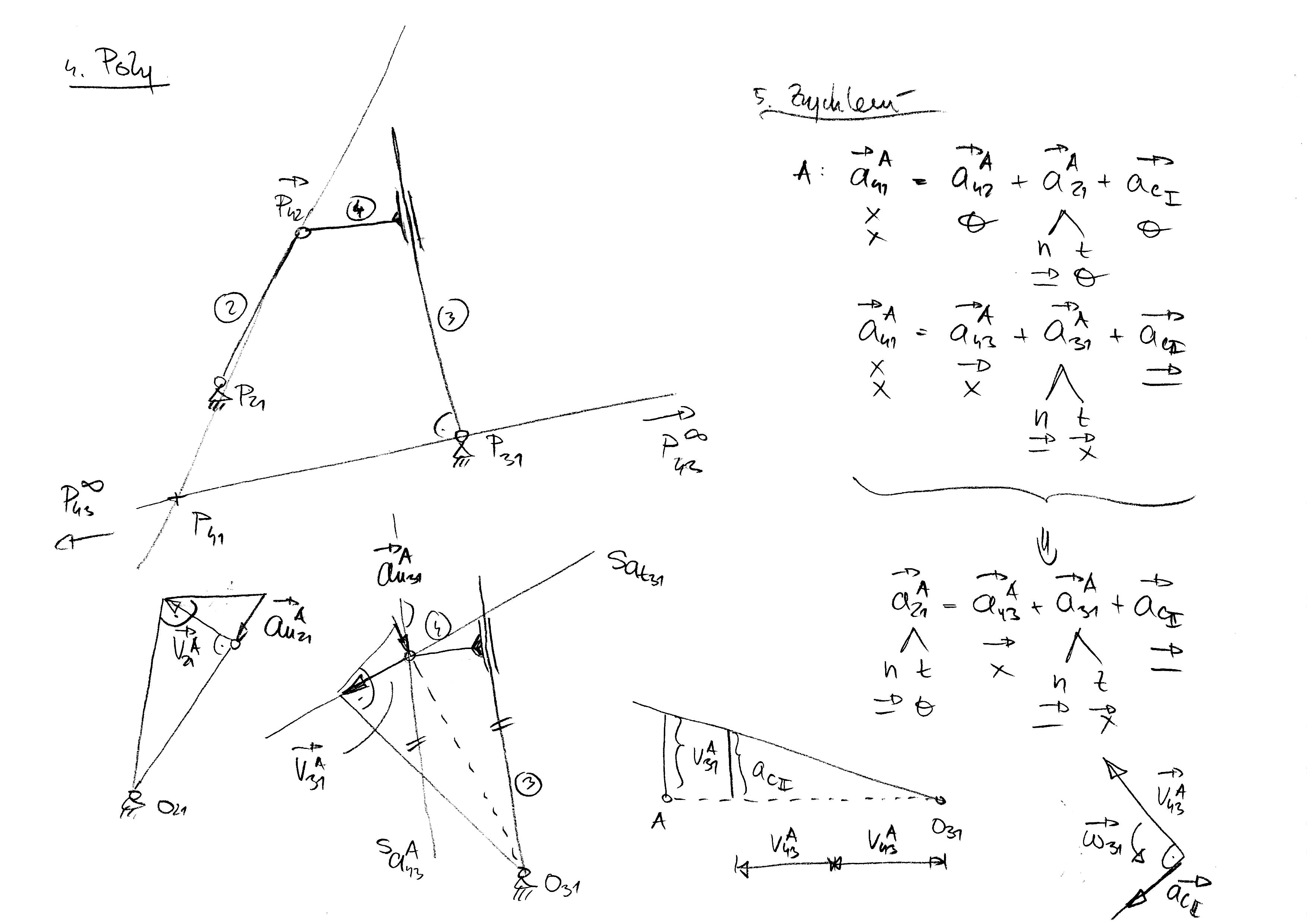
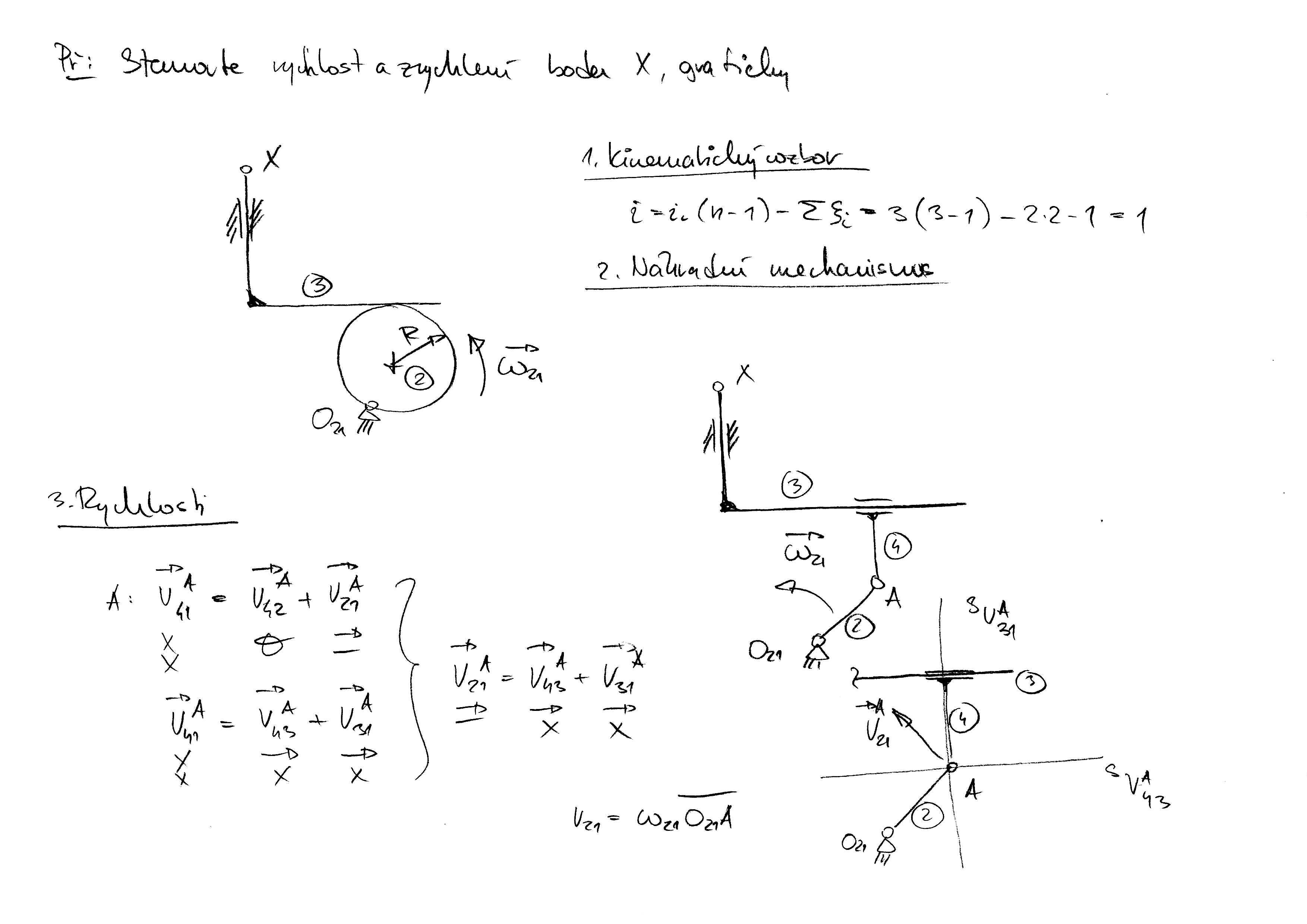
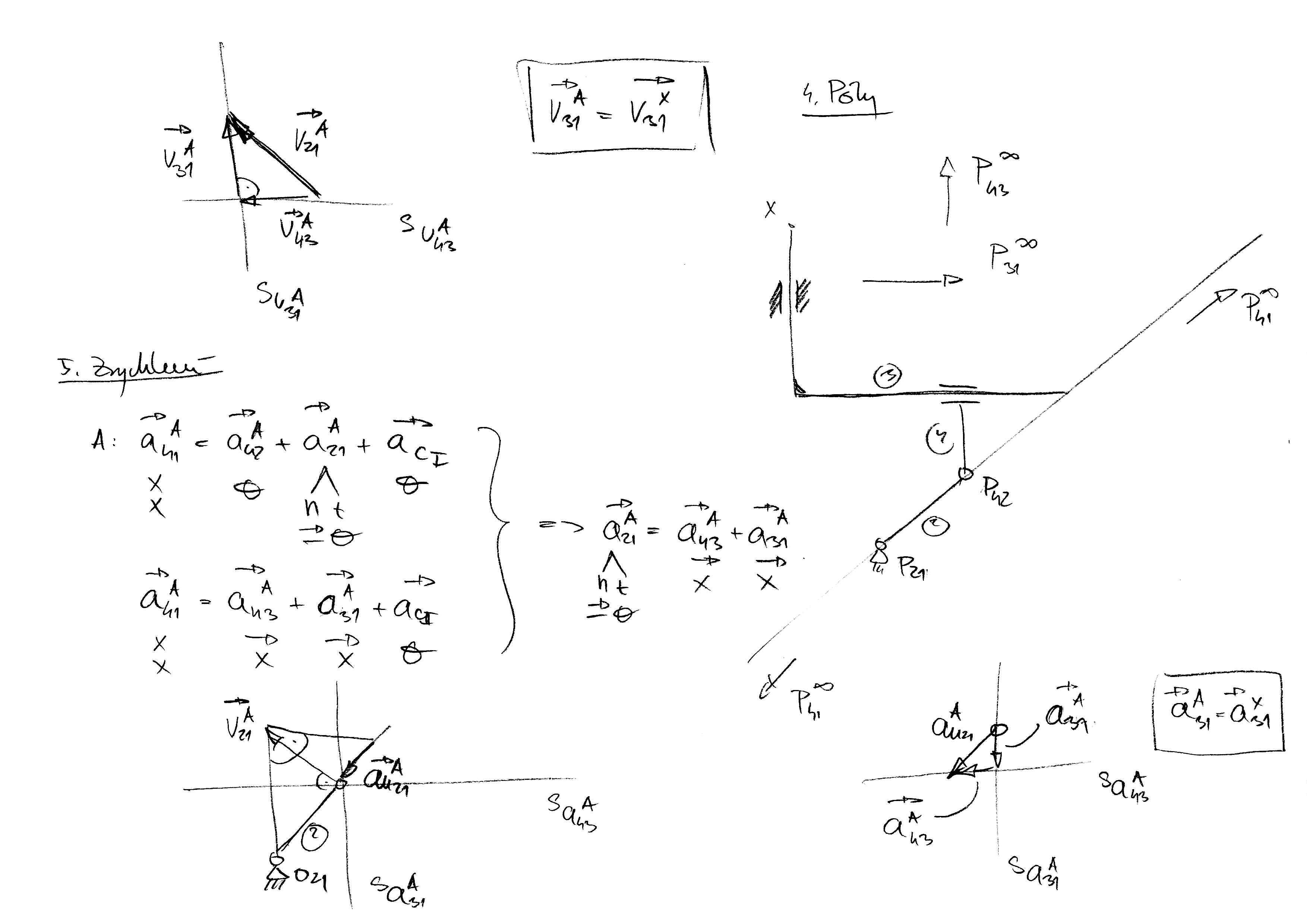
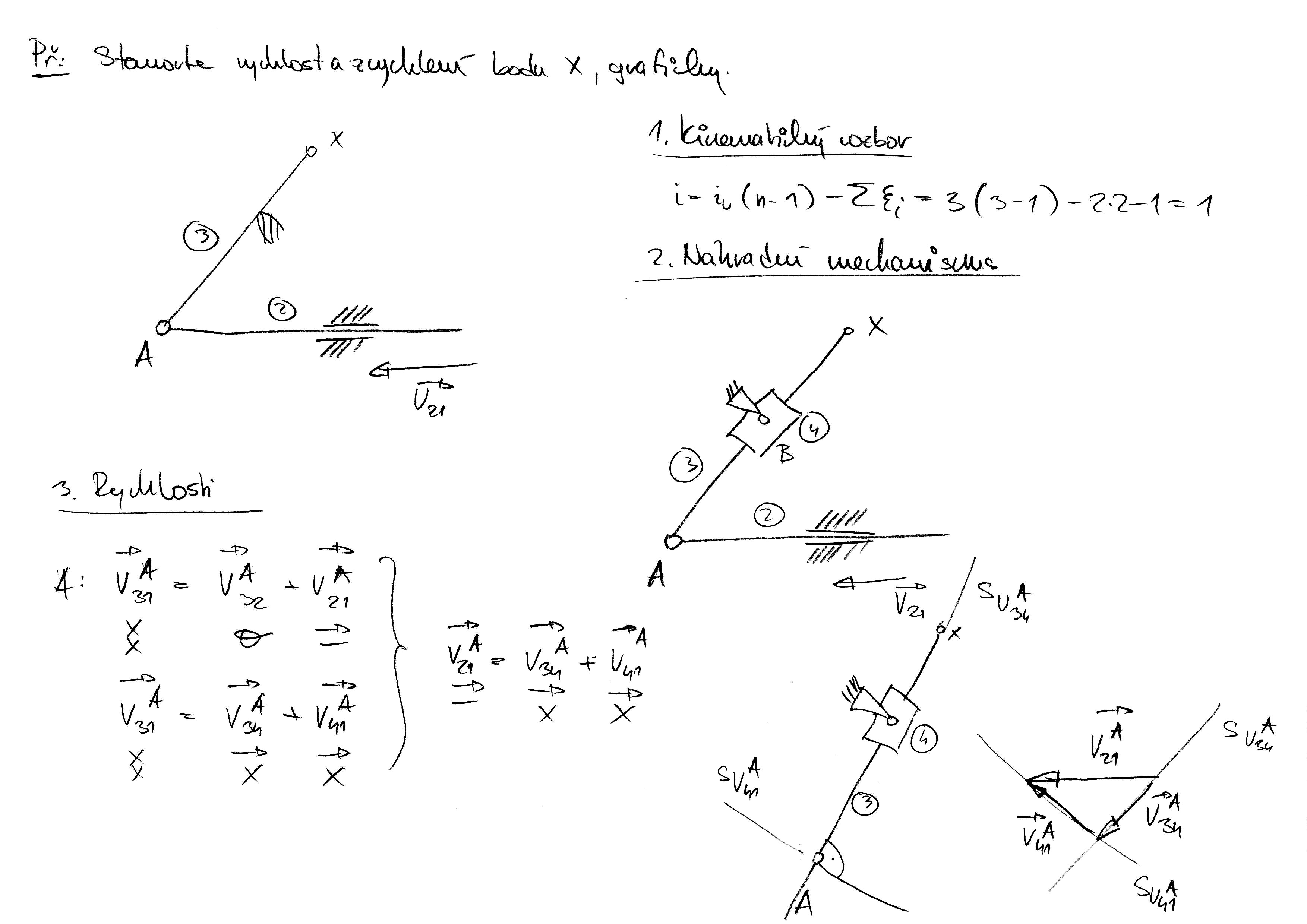
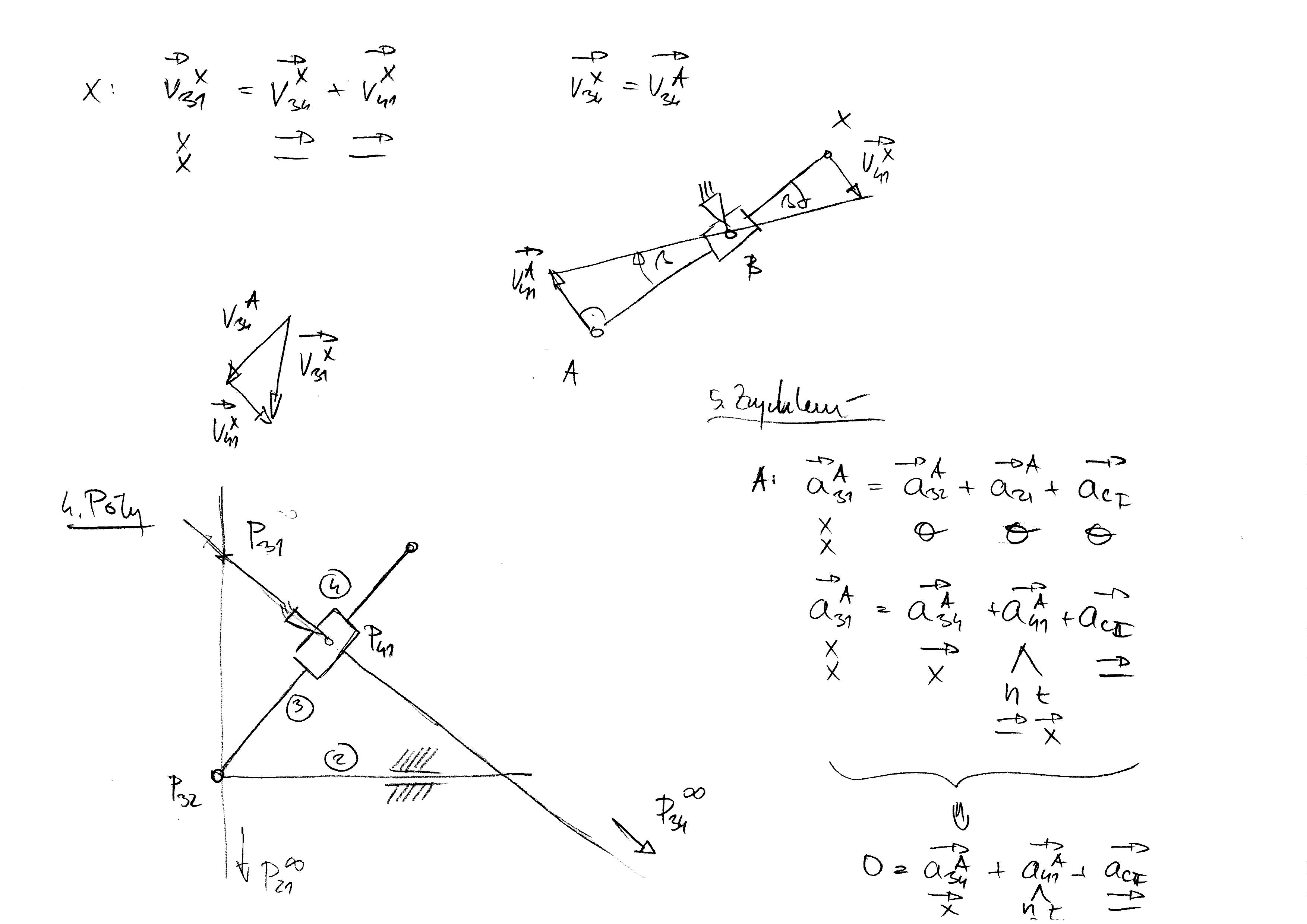
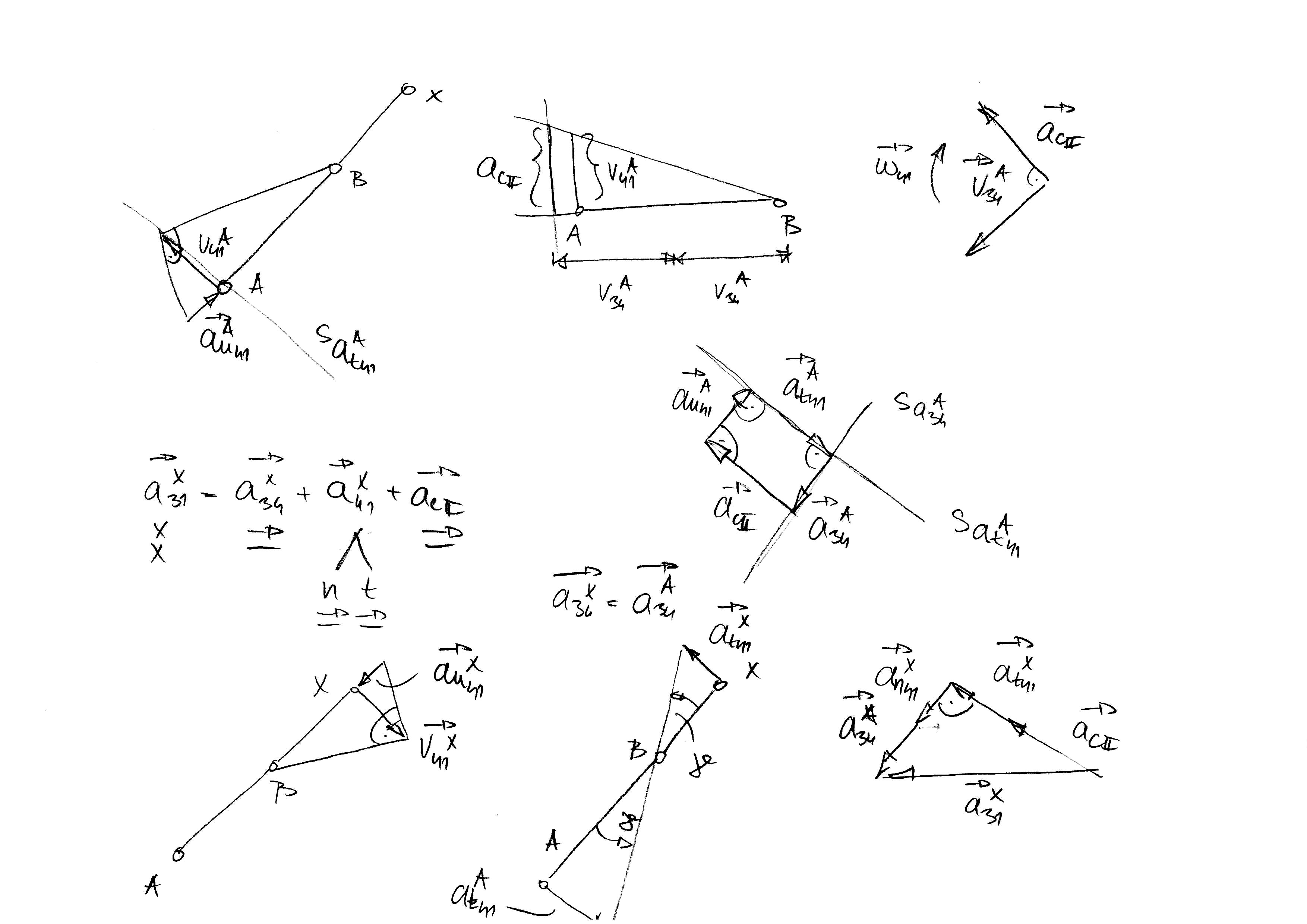
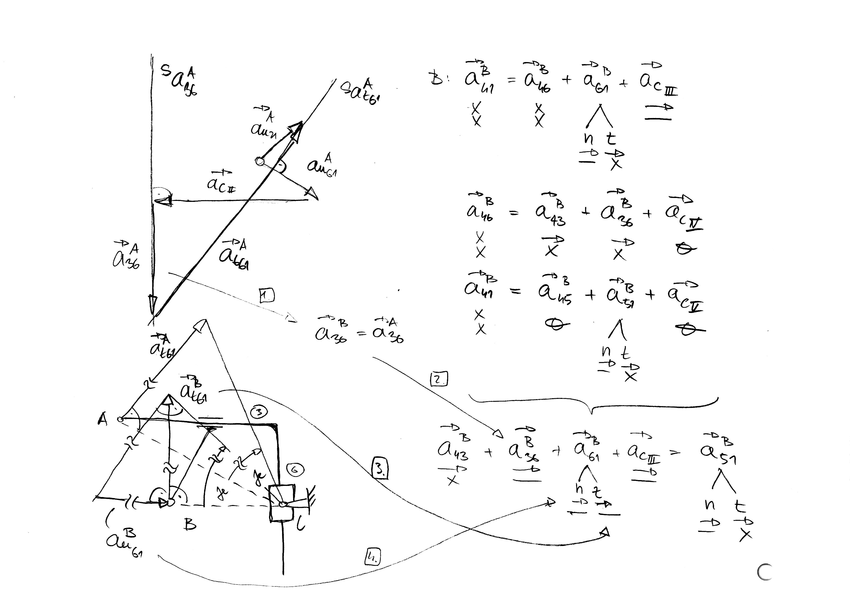
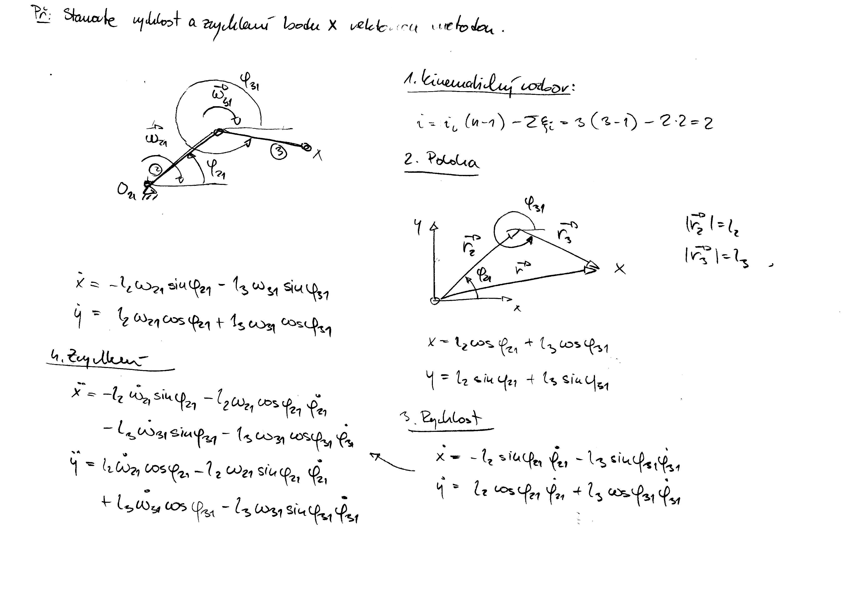
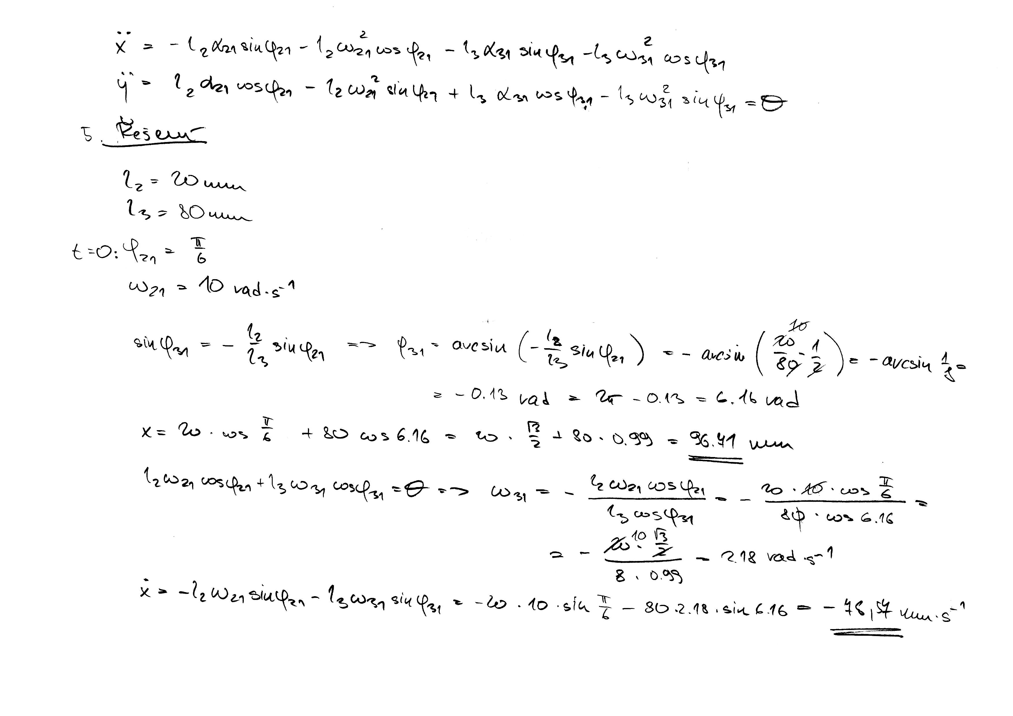
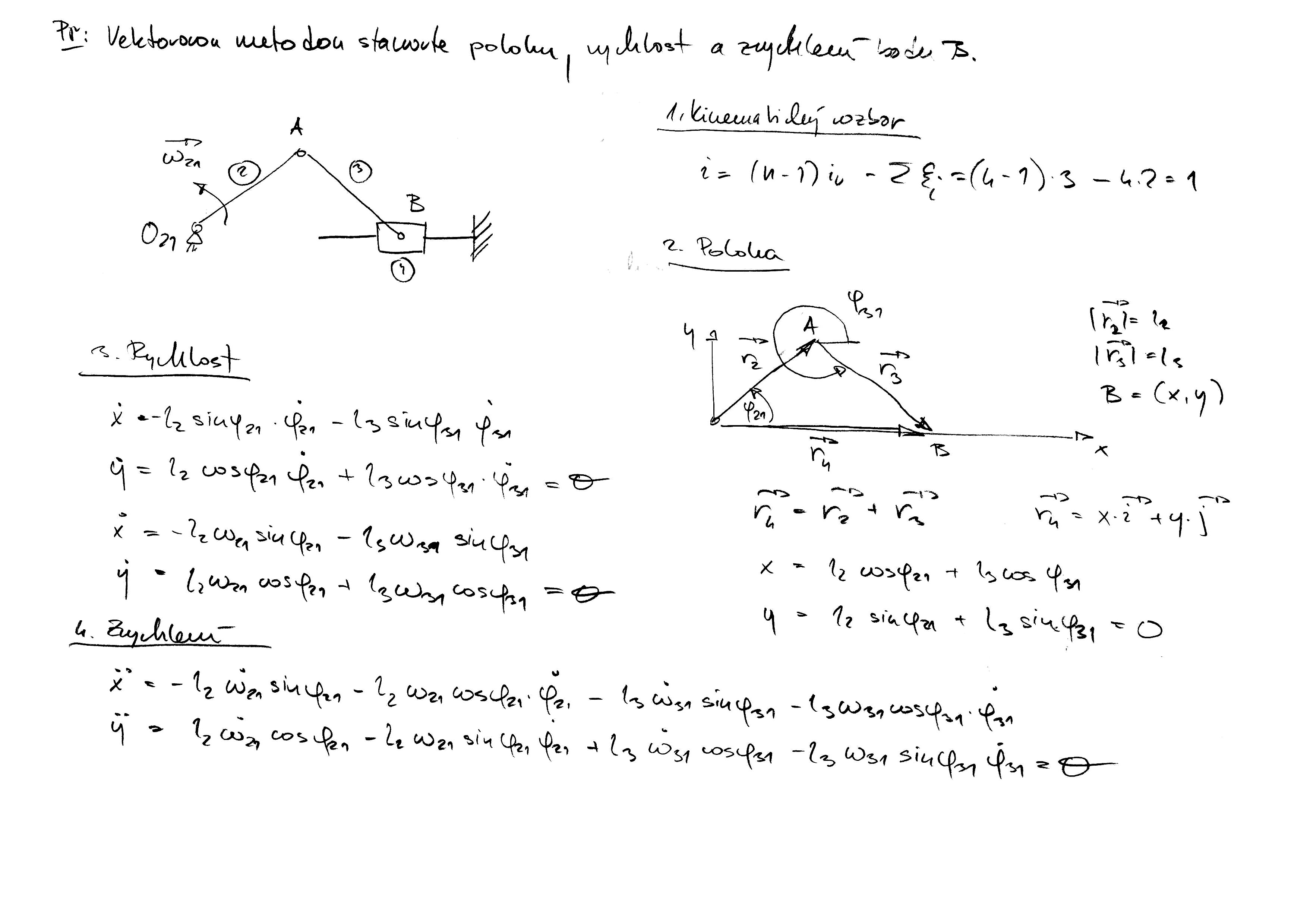
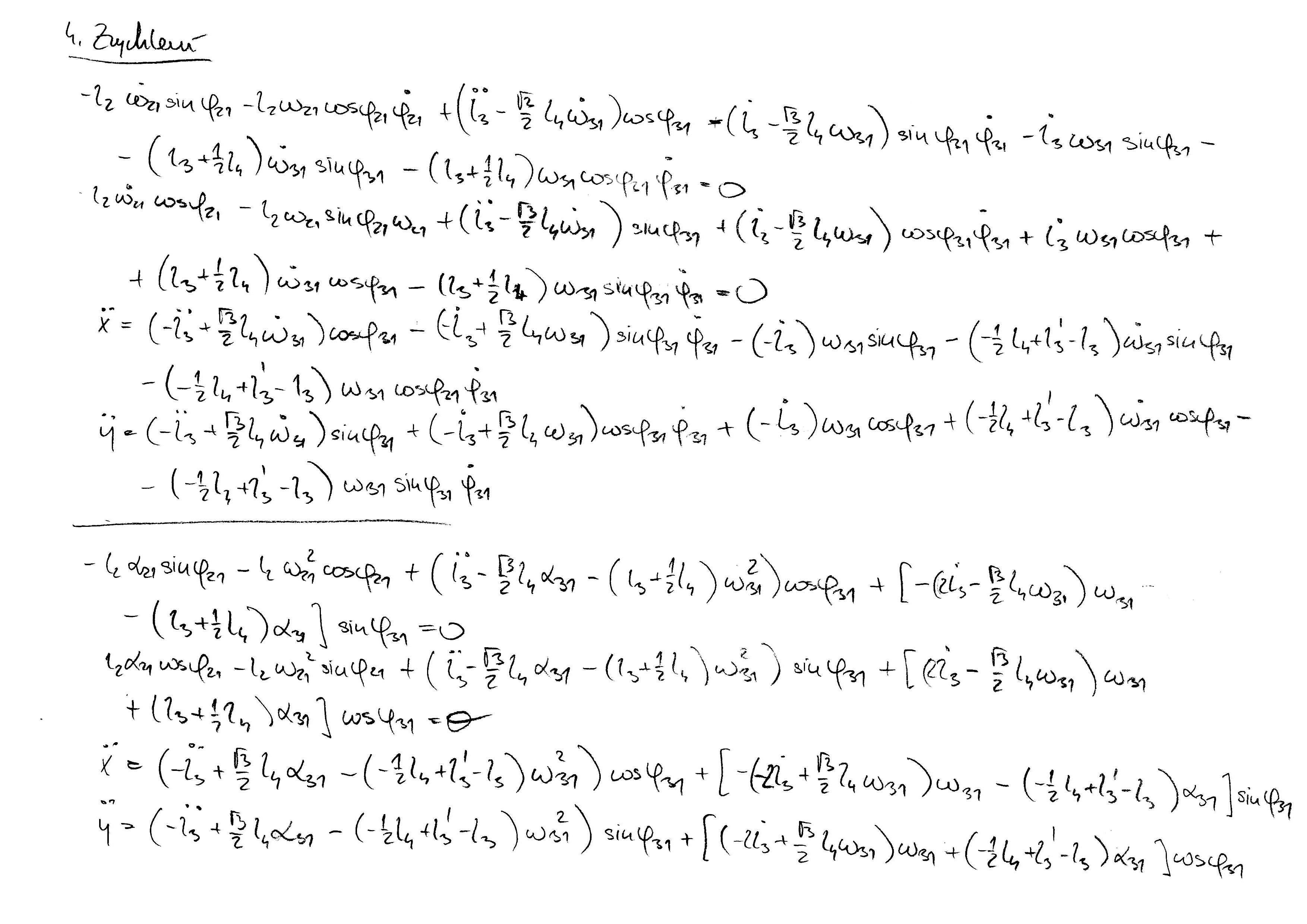
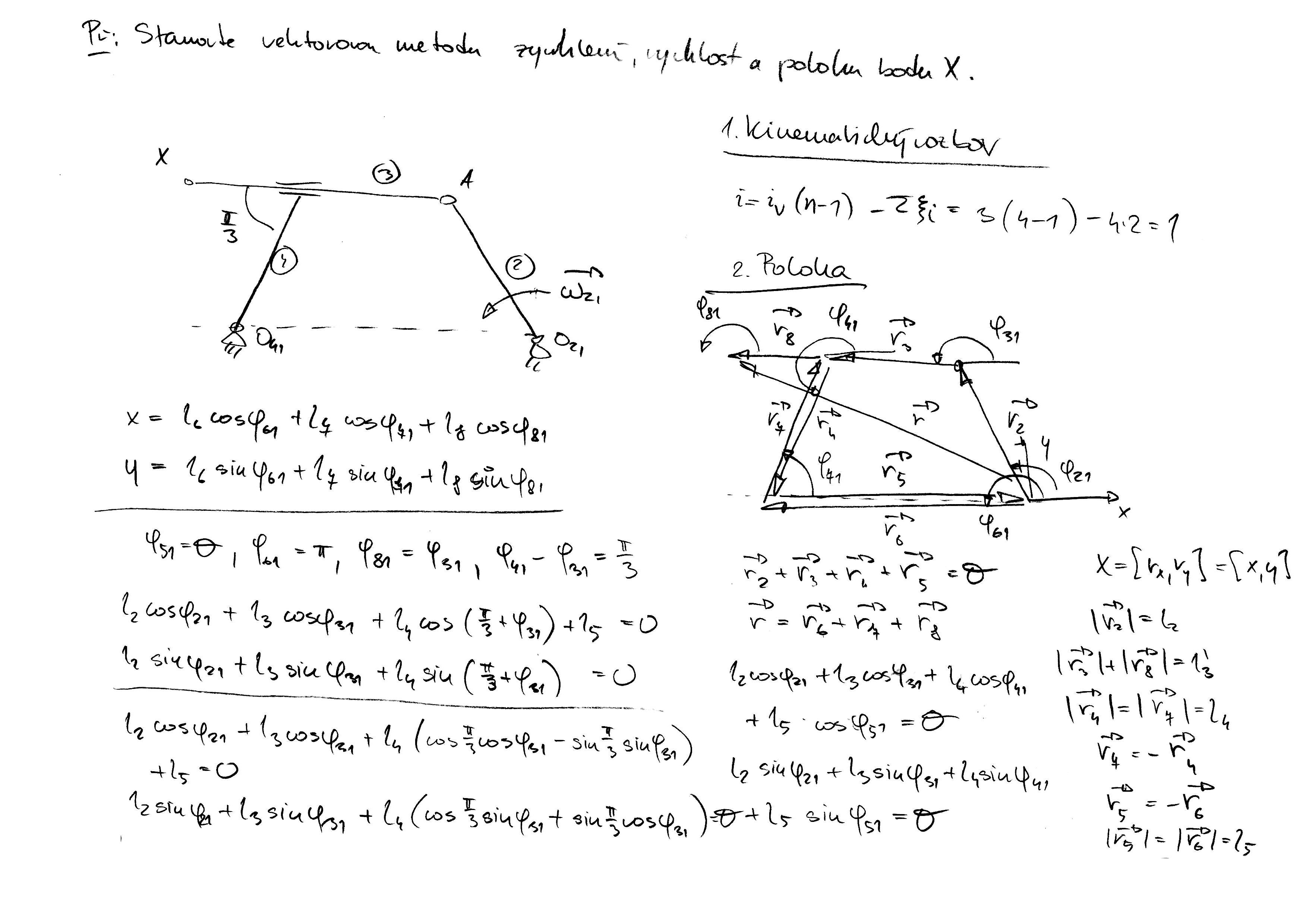
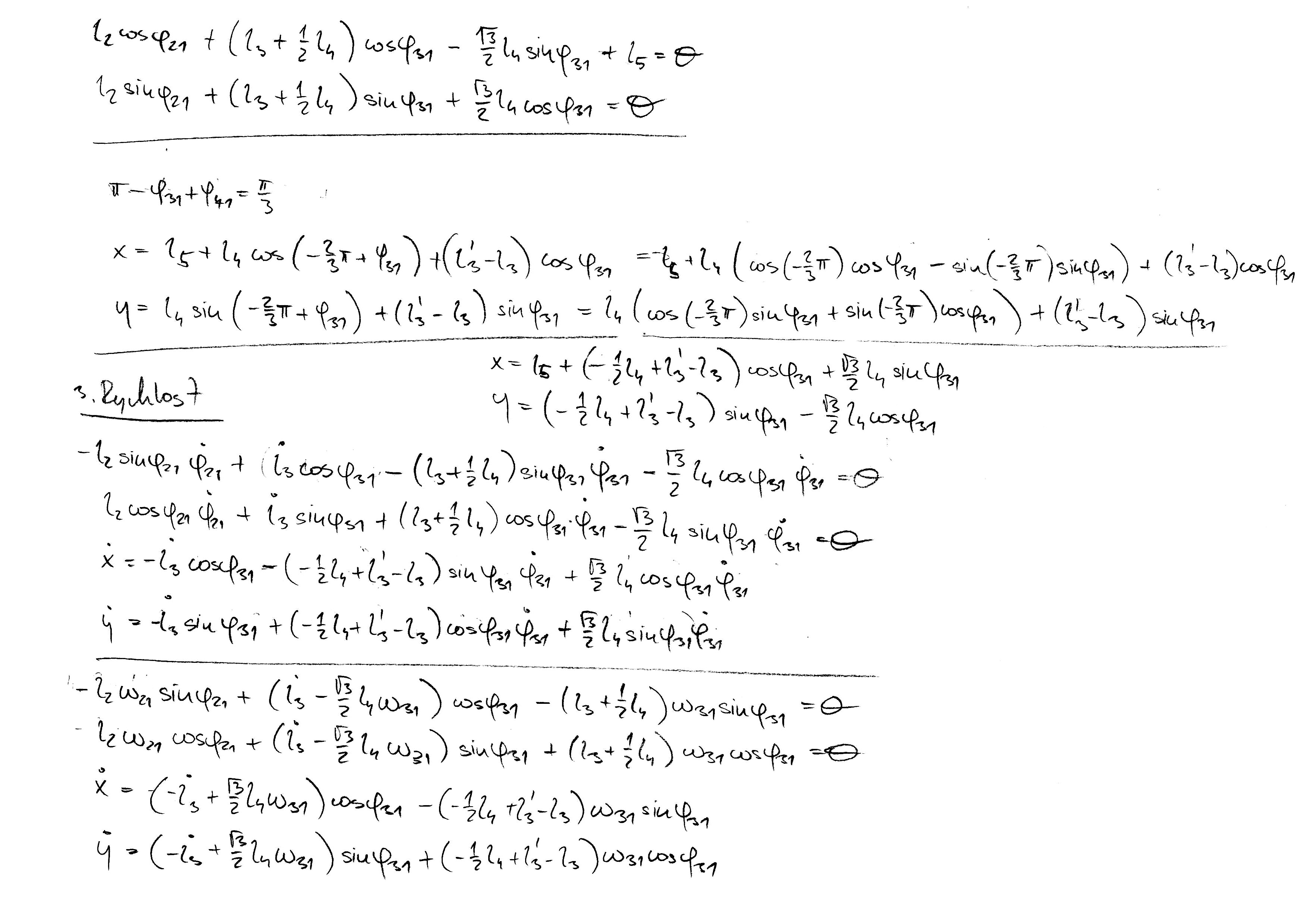
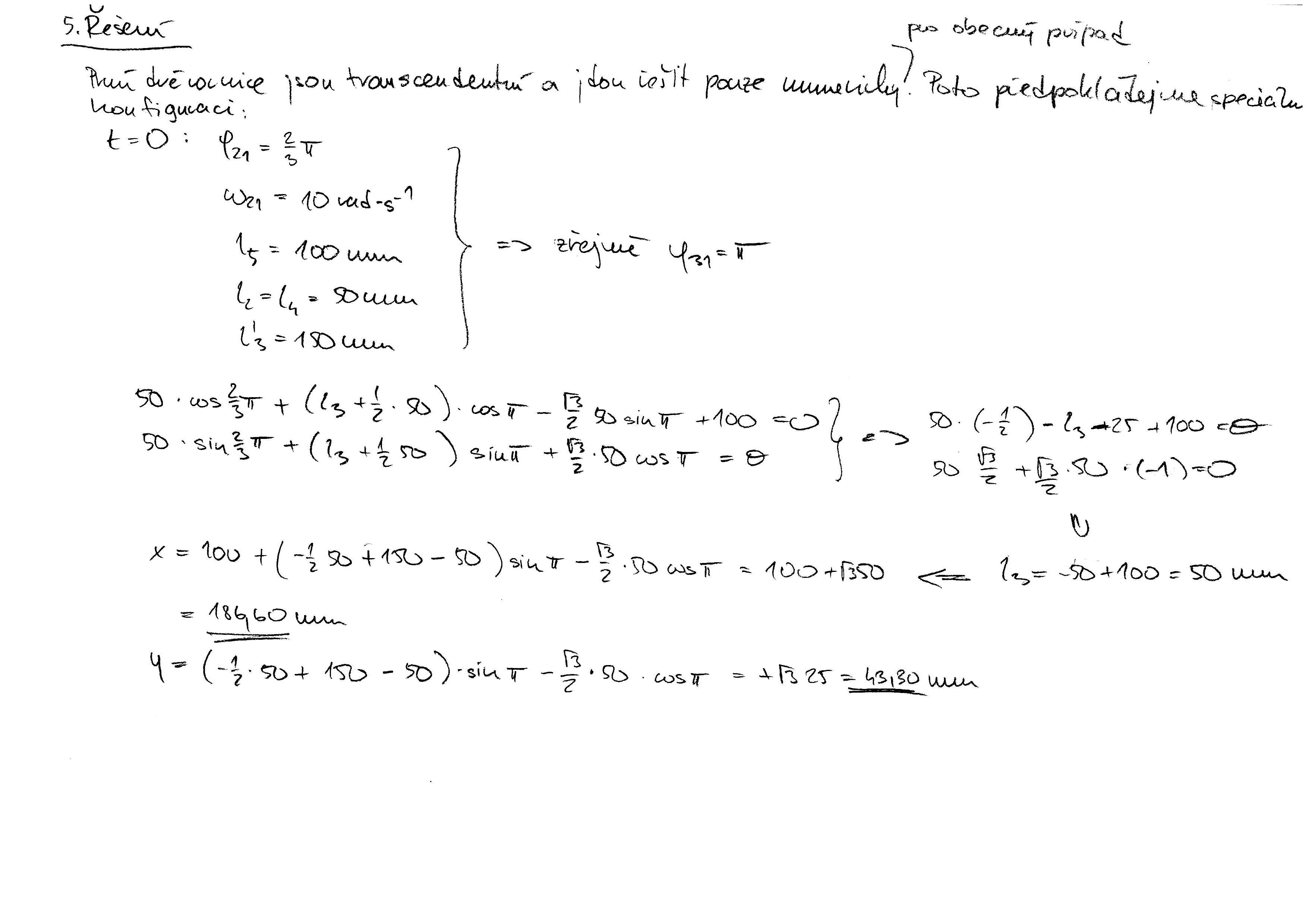
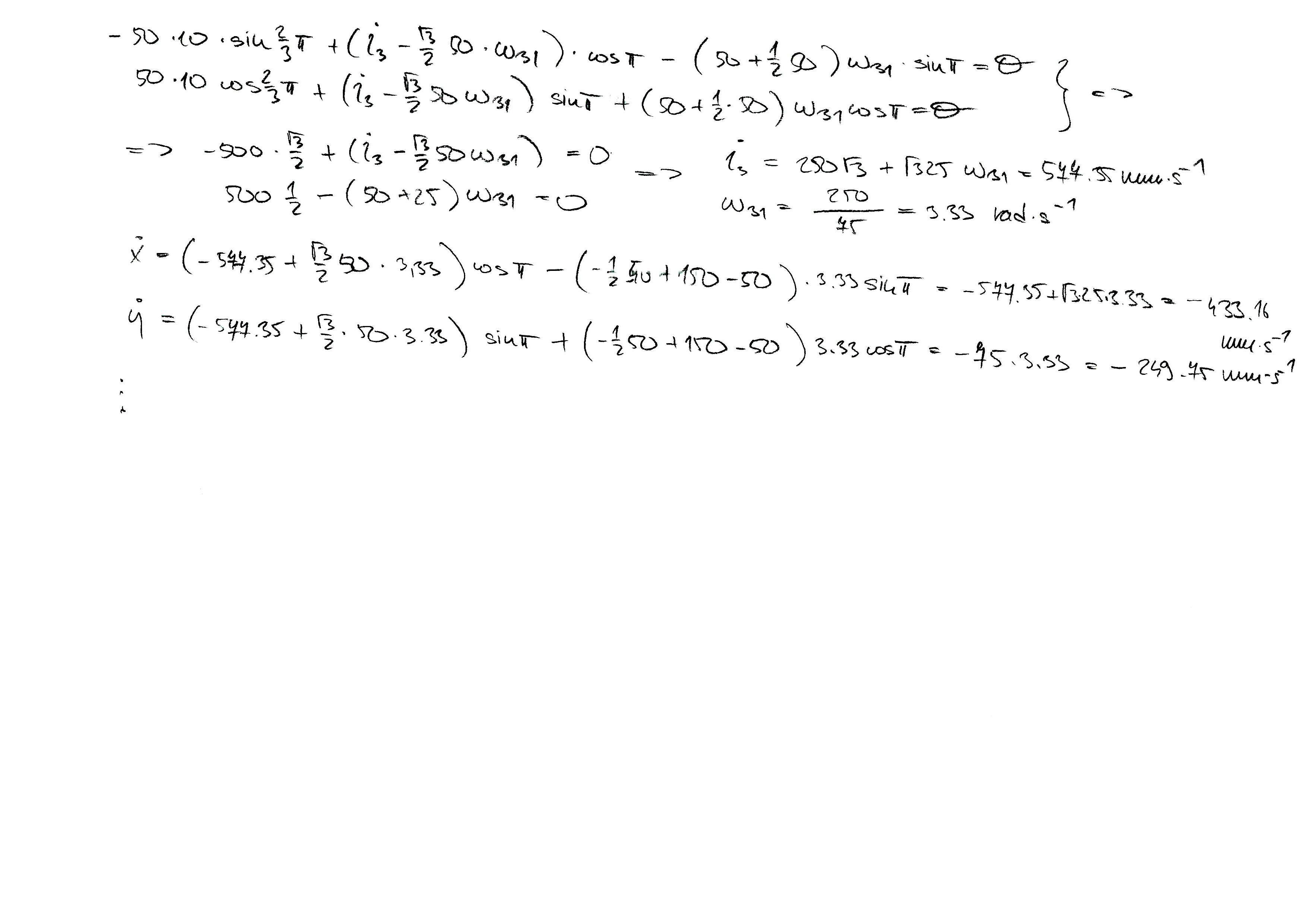
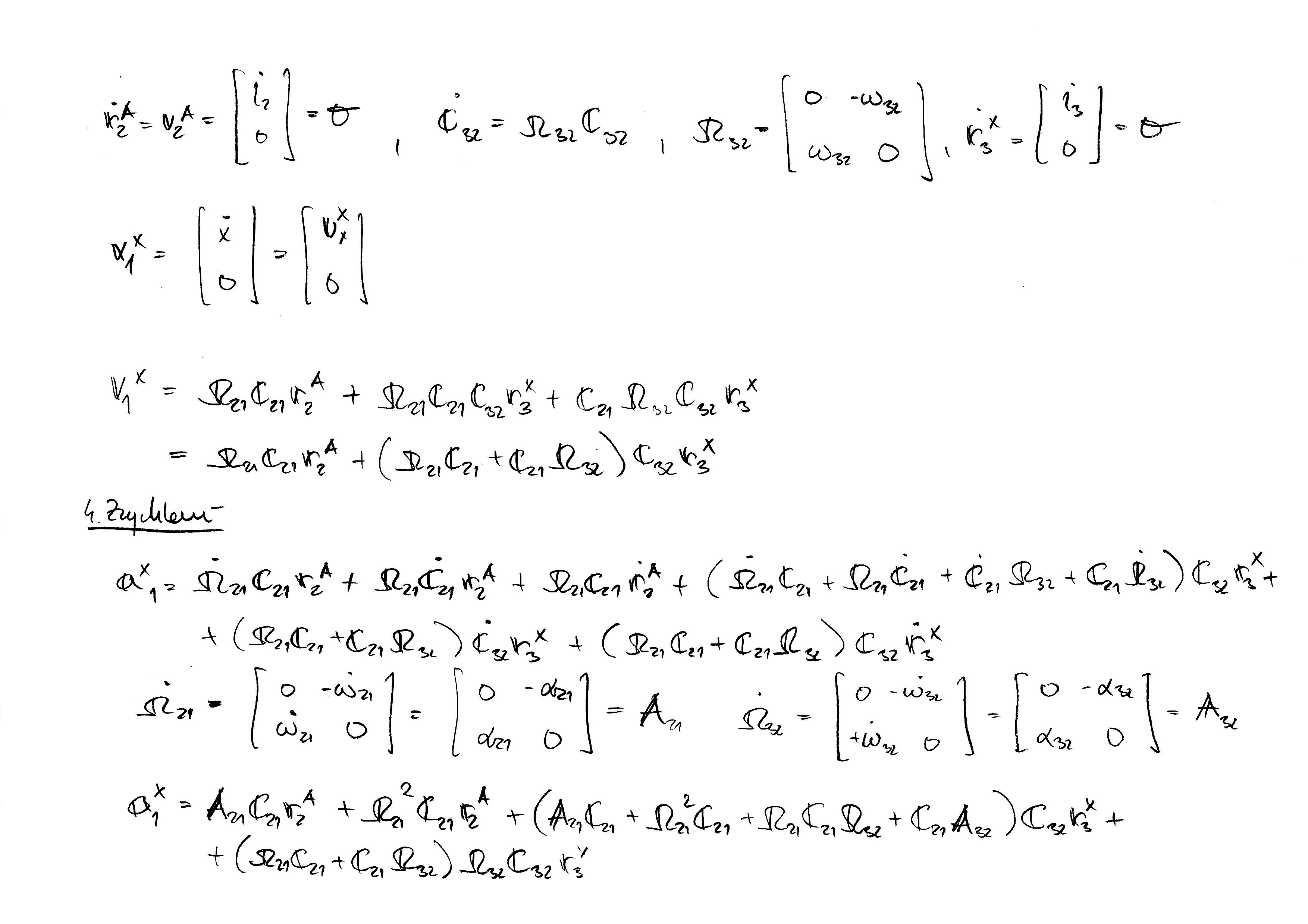
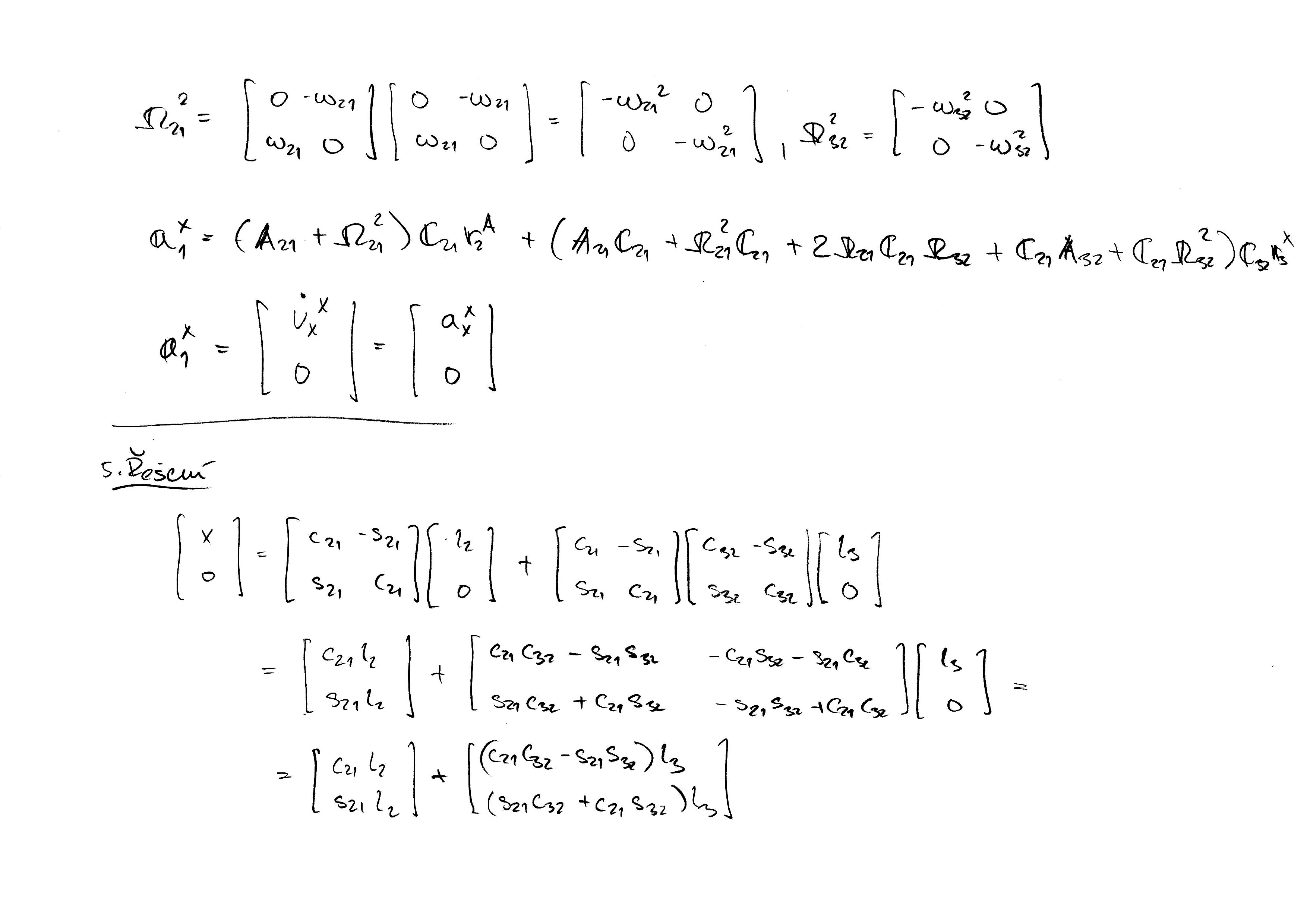
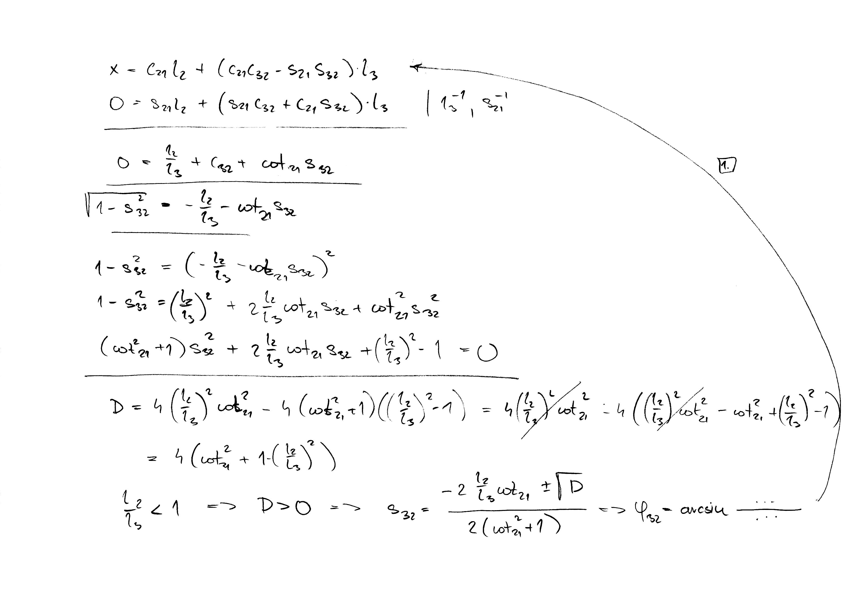
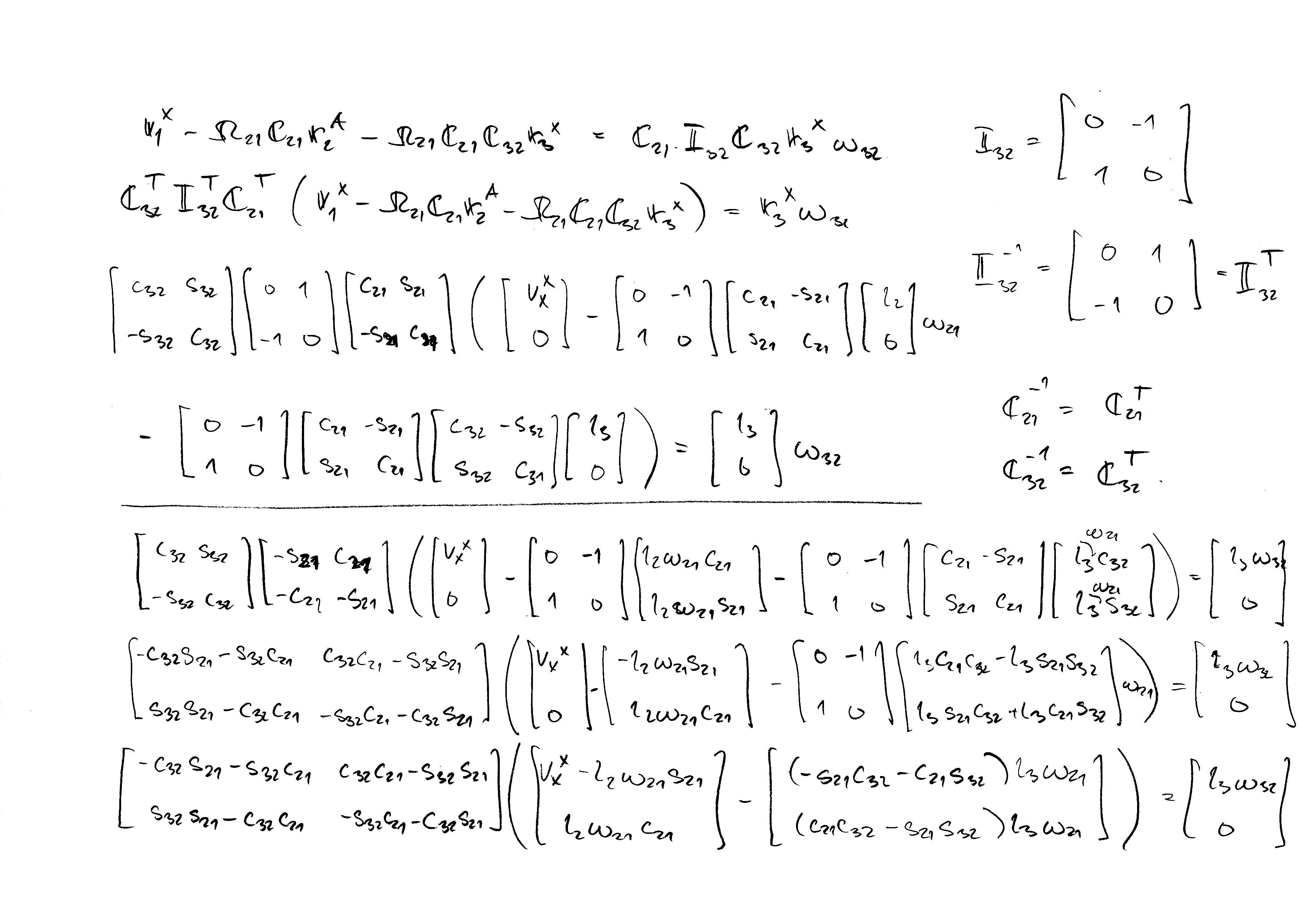
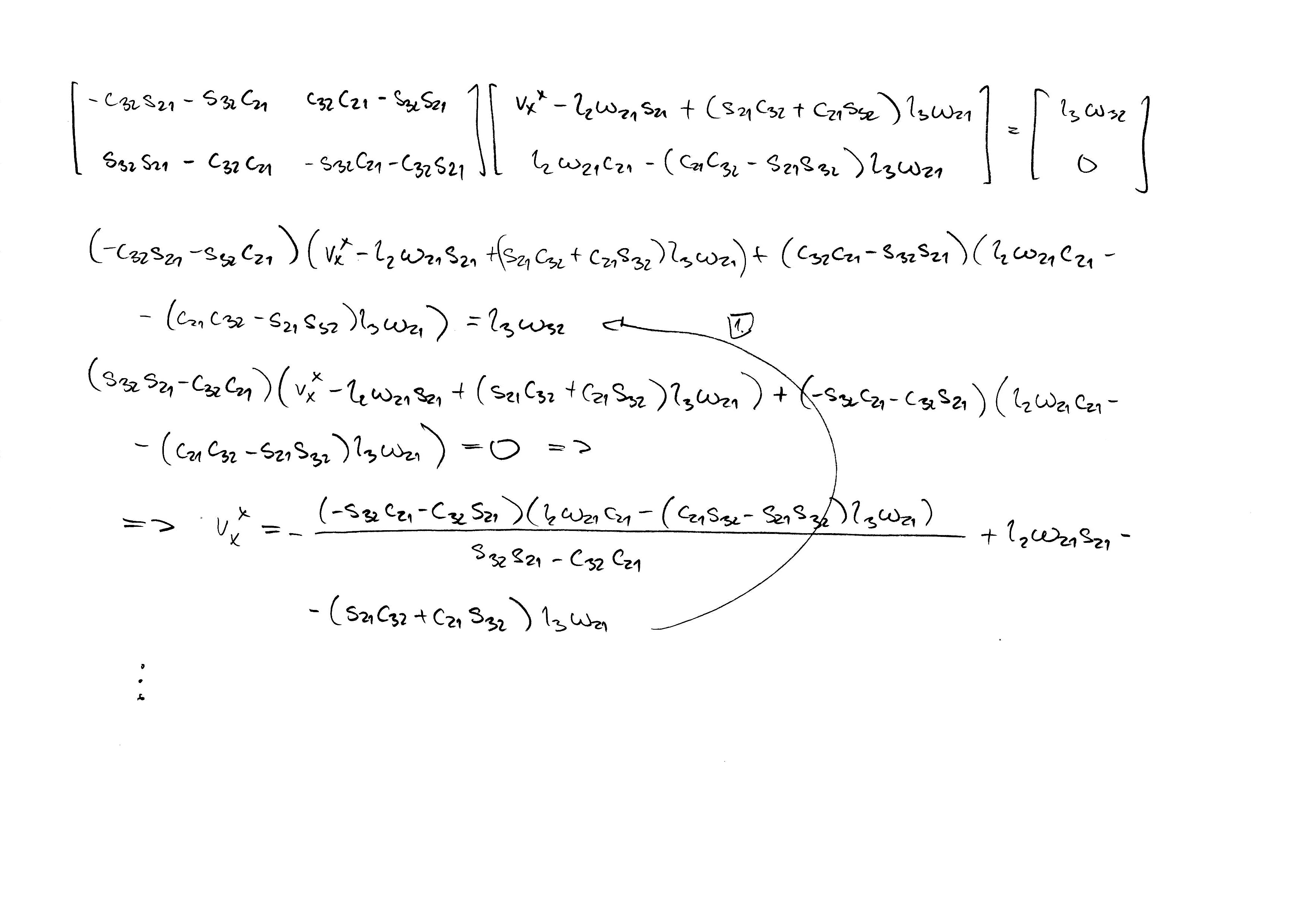
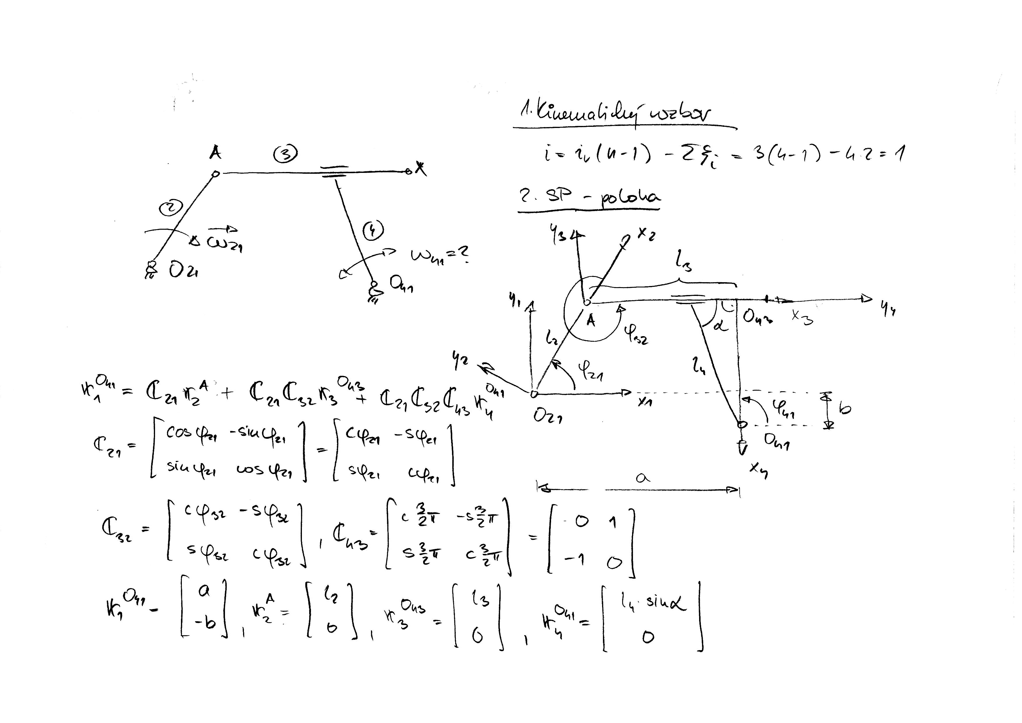
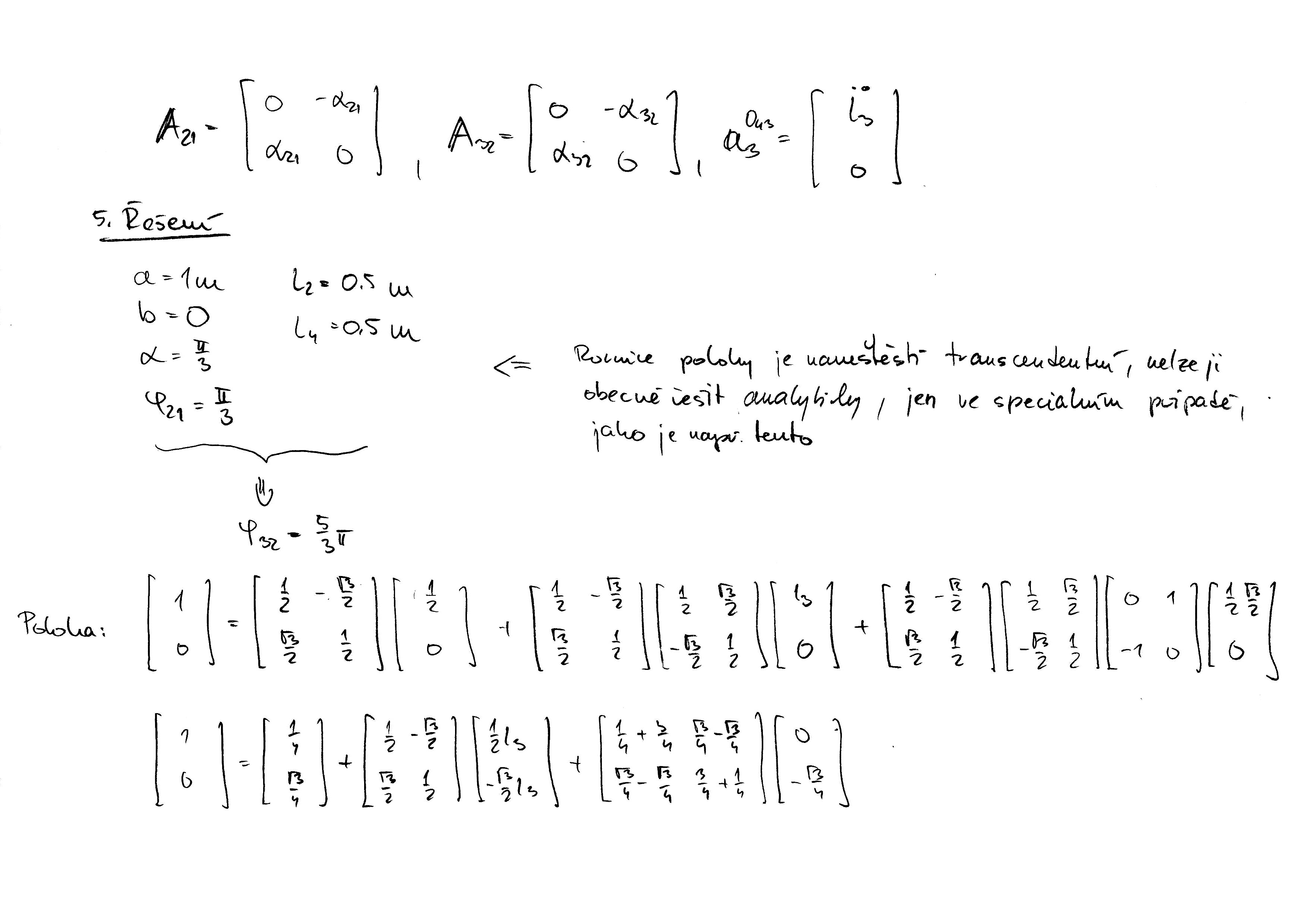
  • Cvičení 4: Obecný rovinný pohyb (ORP).

    • Ručně řešený příklad Př.1 lze stáhnout zde, zde a zde.

    • Ručně řešený příklad Př.2 lze stáhnout zde, zde a zde.

    • Ručně řešený příklad Př.3 lze stáhnout zde, zde, zde a zde.

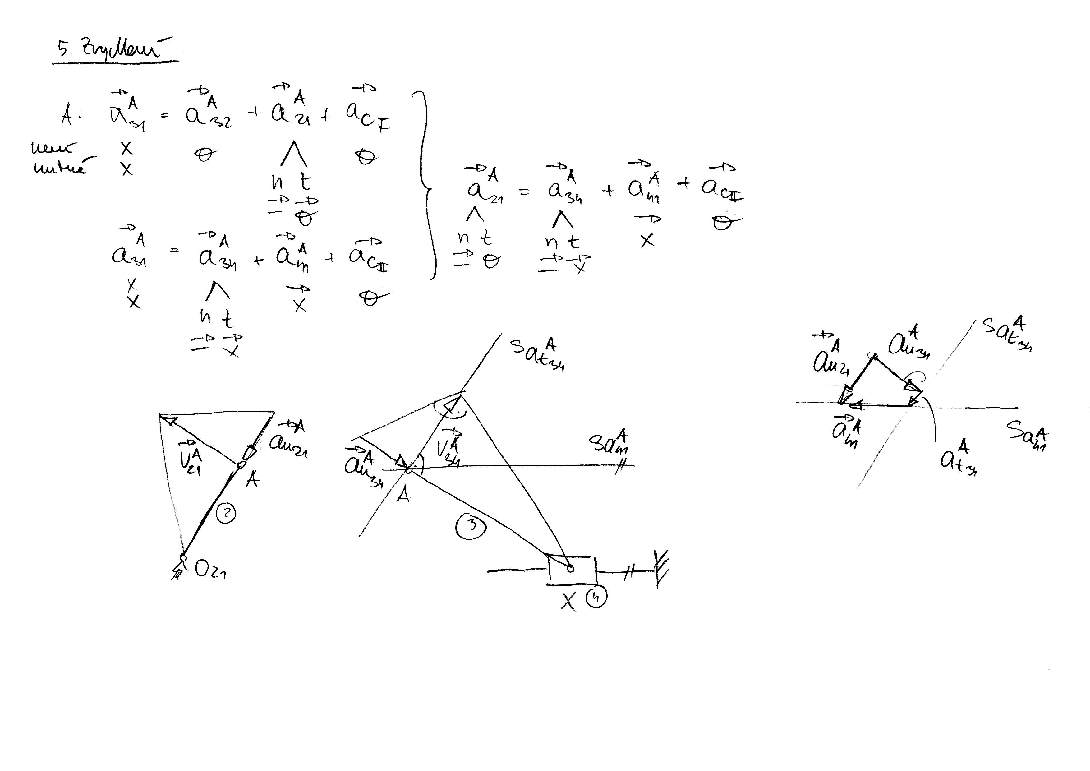
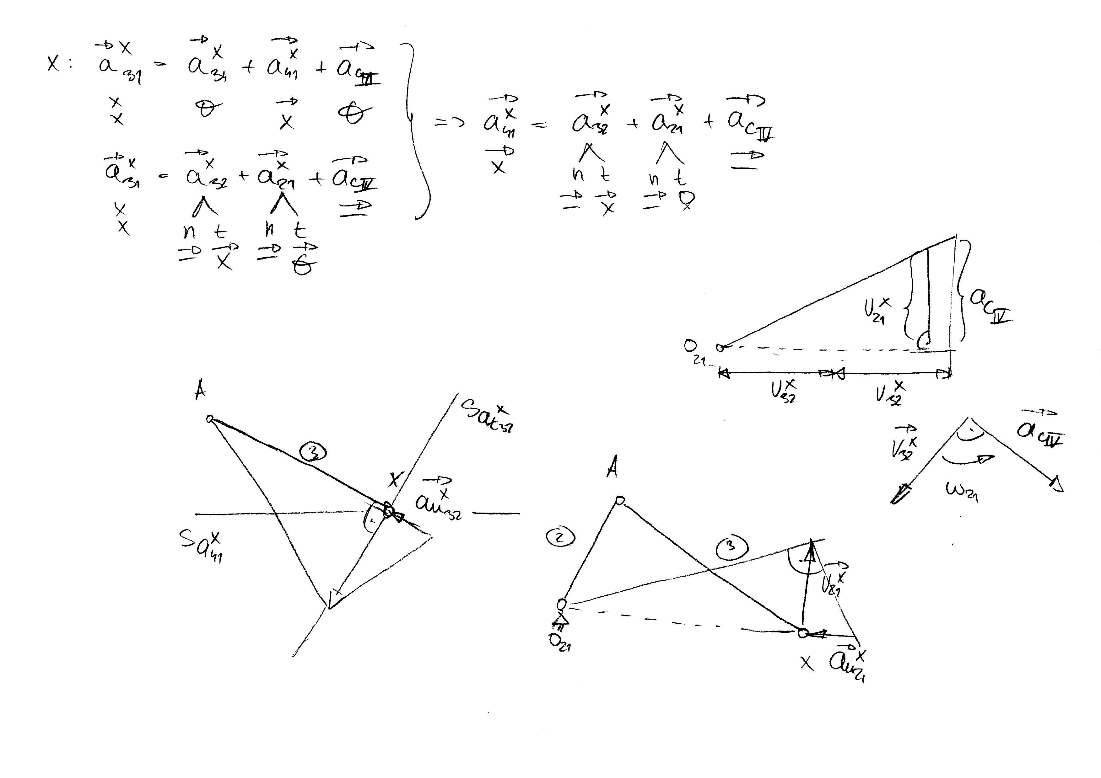
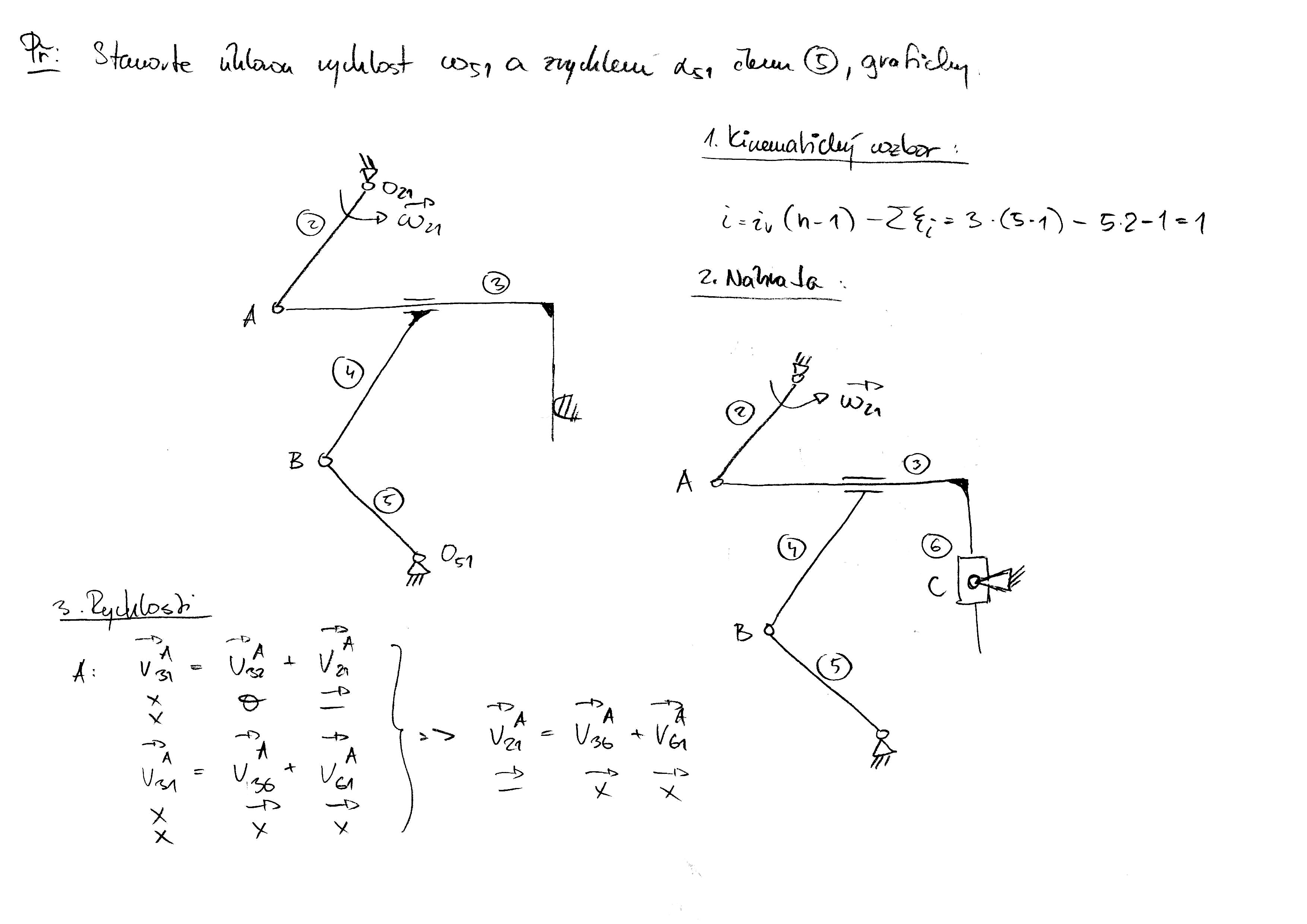
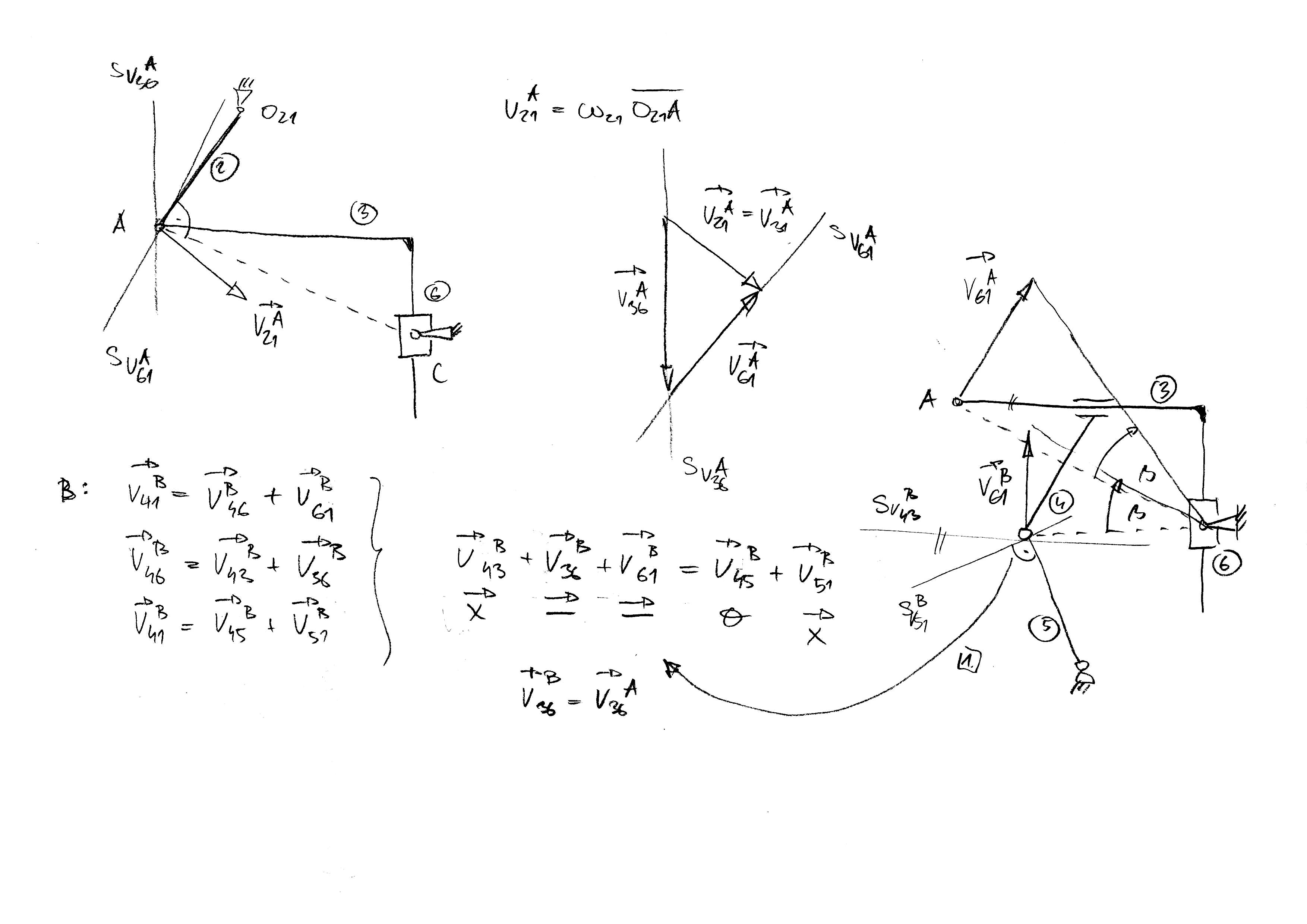
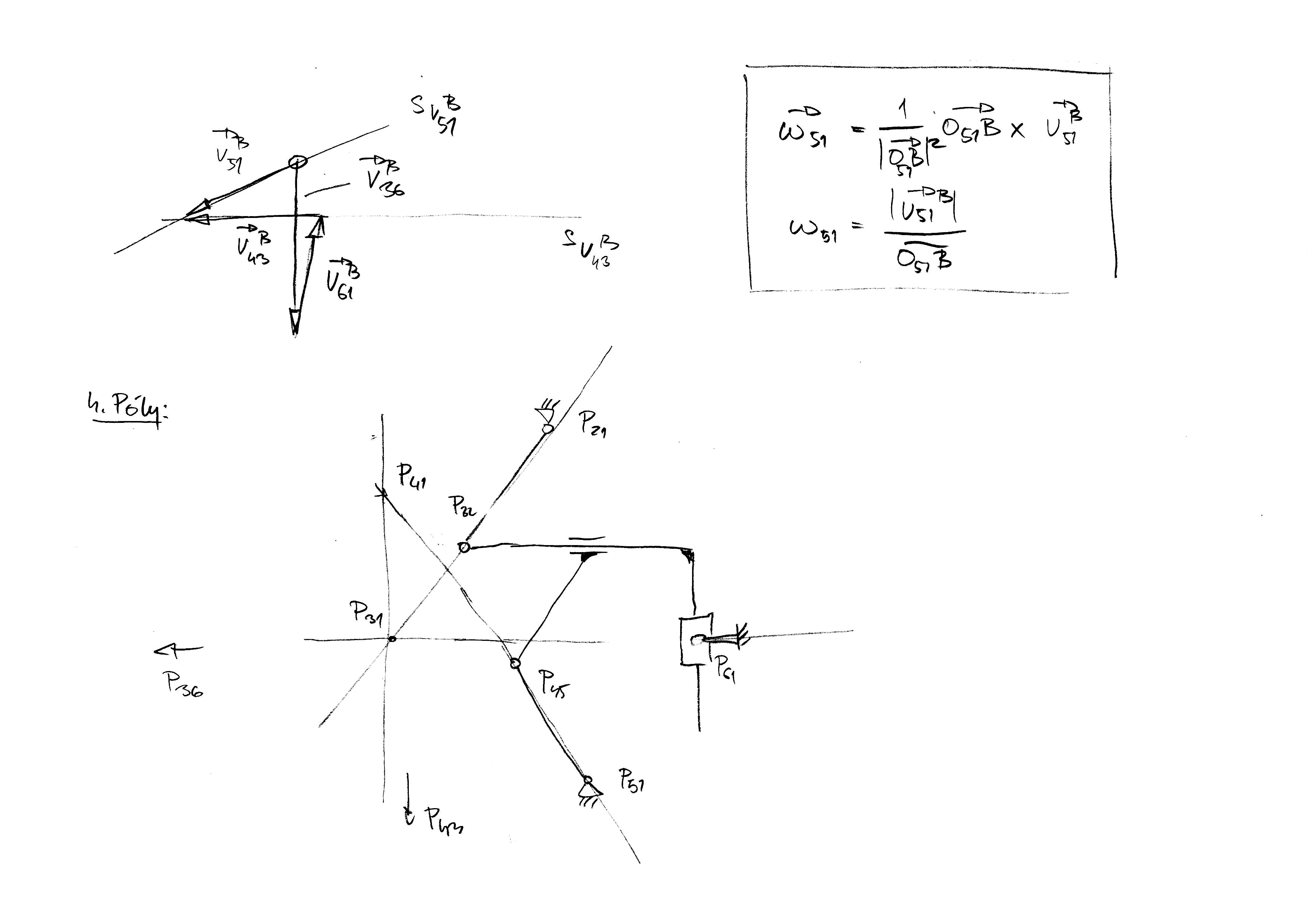
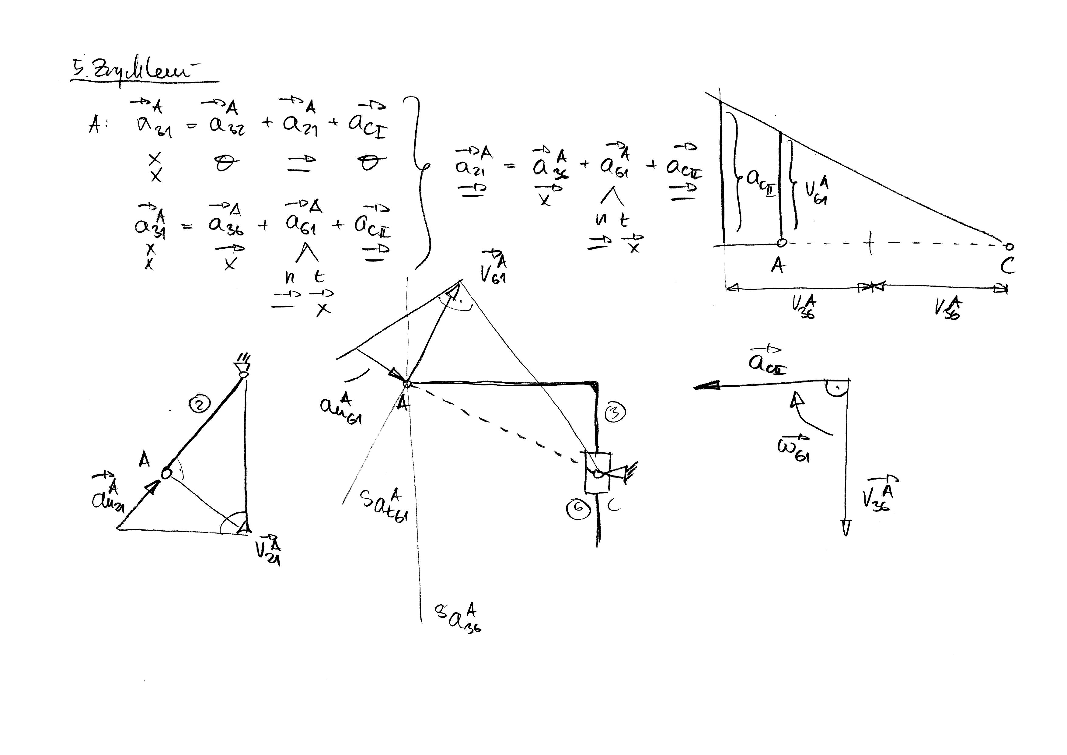
  • Cvičení 5: Obecný rovinný pohyb (ORP).

    • Ručně řešený příklad Př.1 lze stáhnout zde, zde a zde.

    • Ručně řešený příklad Př.2 lze stáhnout zde a zde.

    • Ručně řešený příklad Př.3 lze stáhnout zde, zde a zde.

    • Ručně řešený příklad Př.4 lze stáhnout zde, zde a zde.

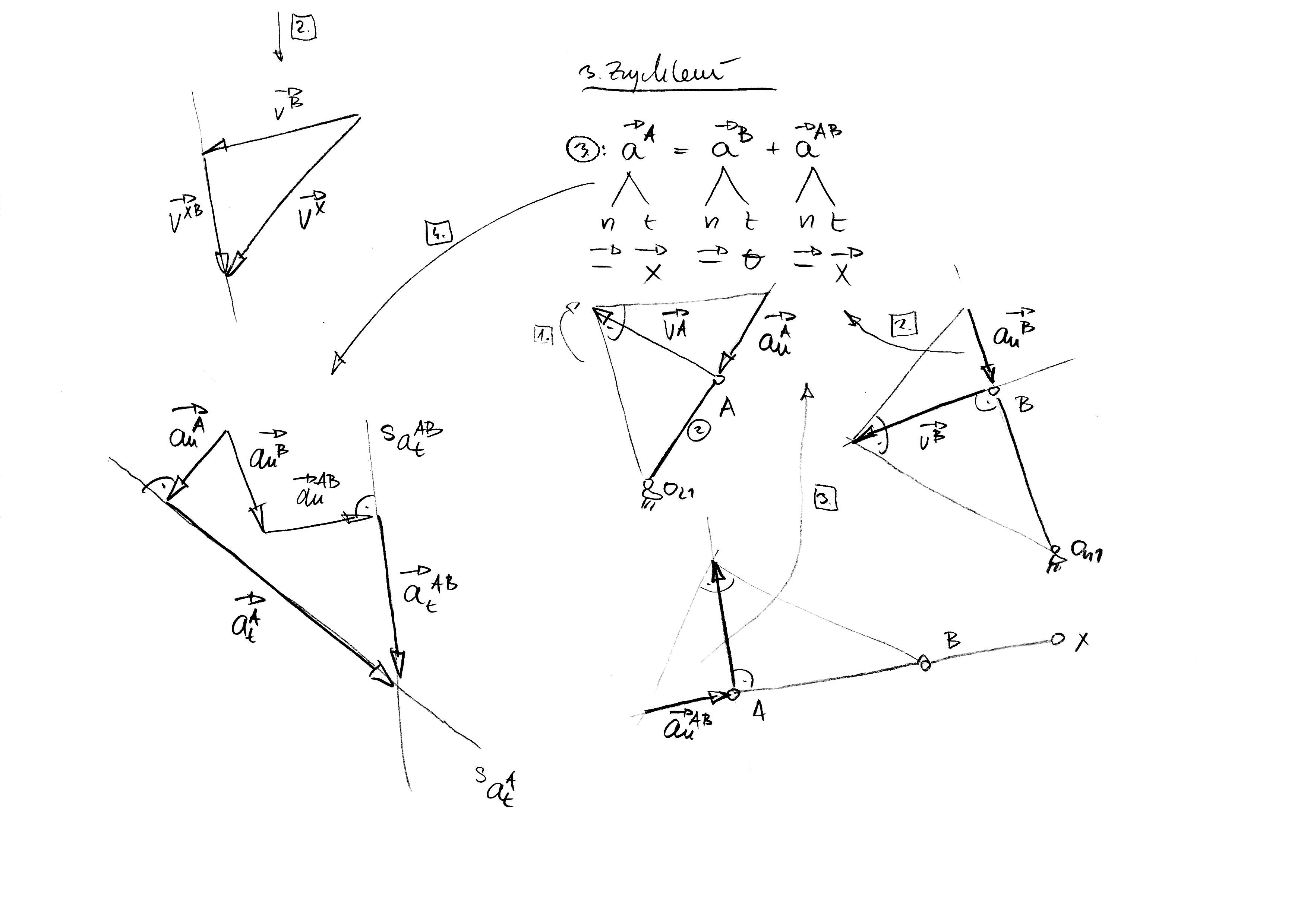
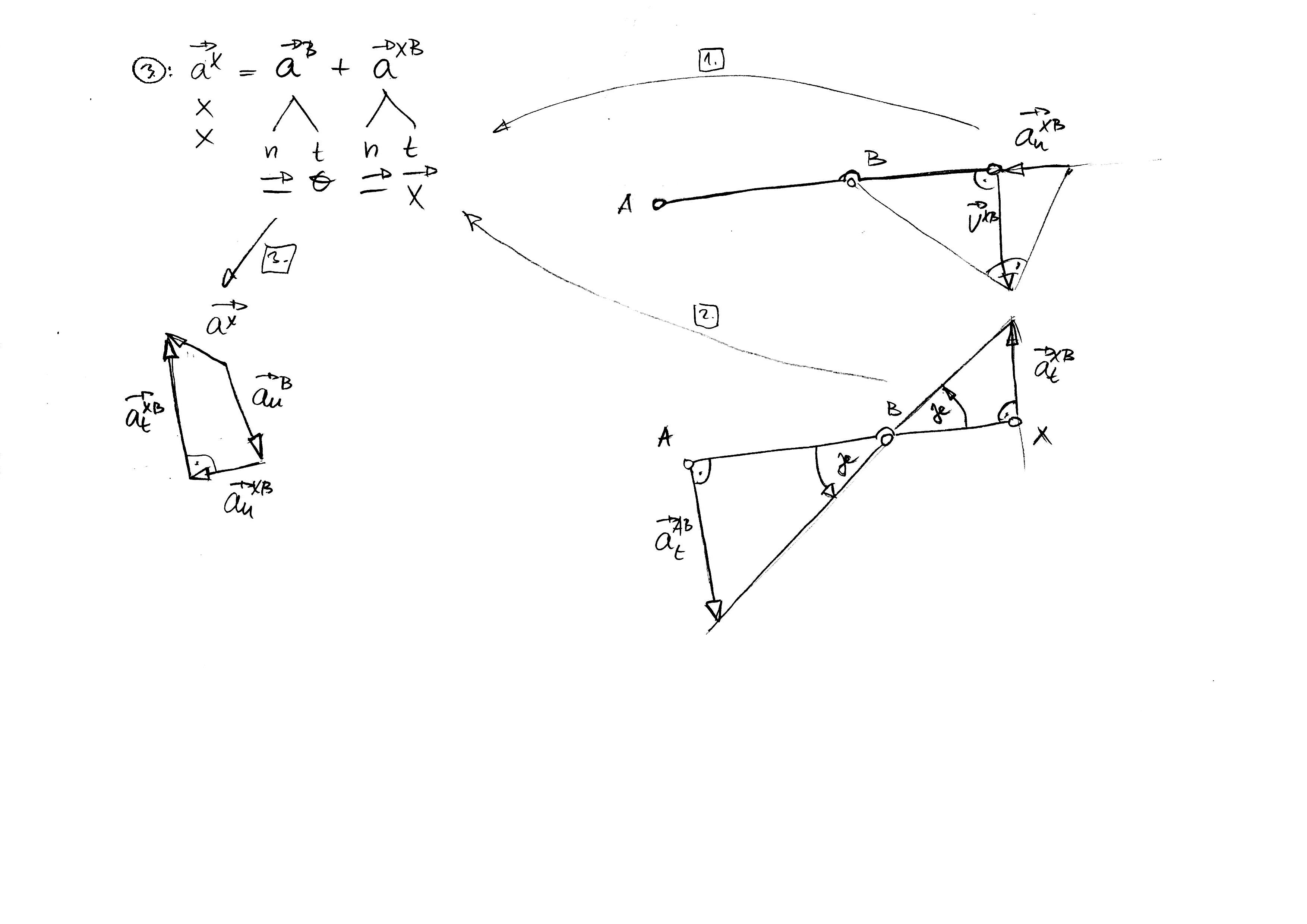
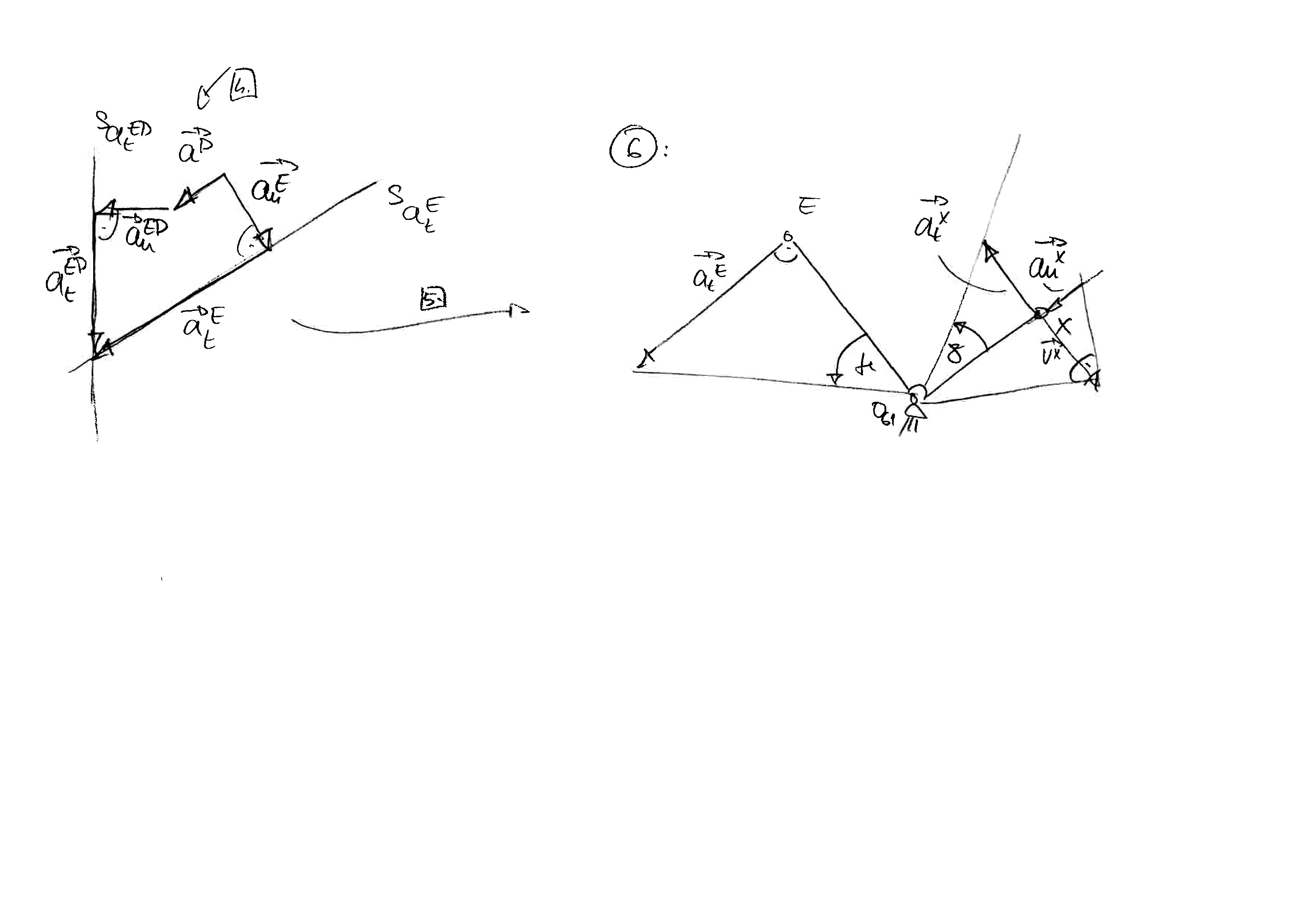
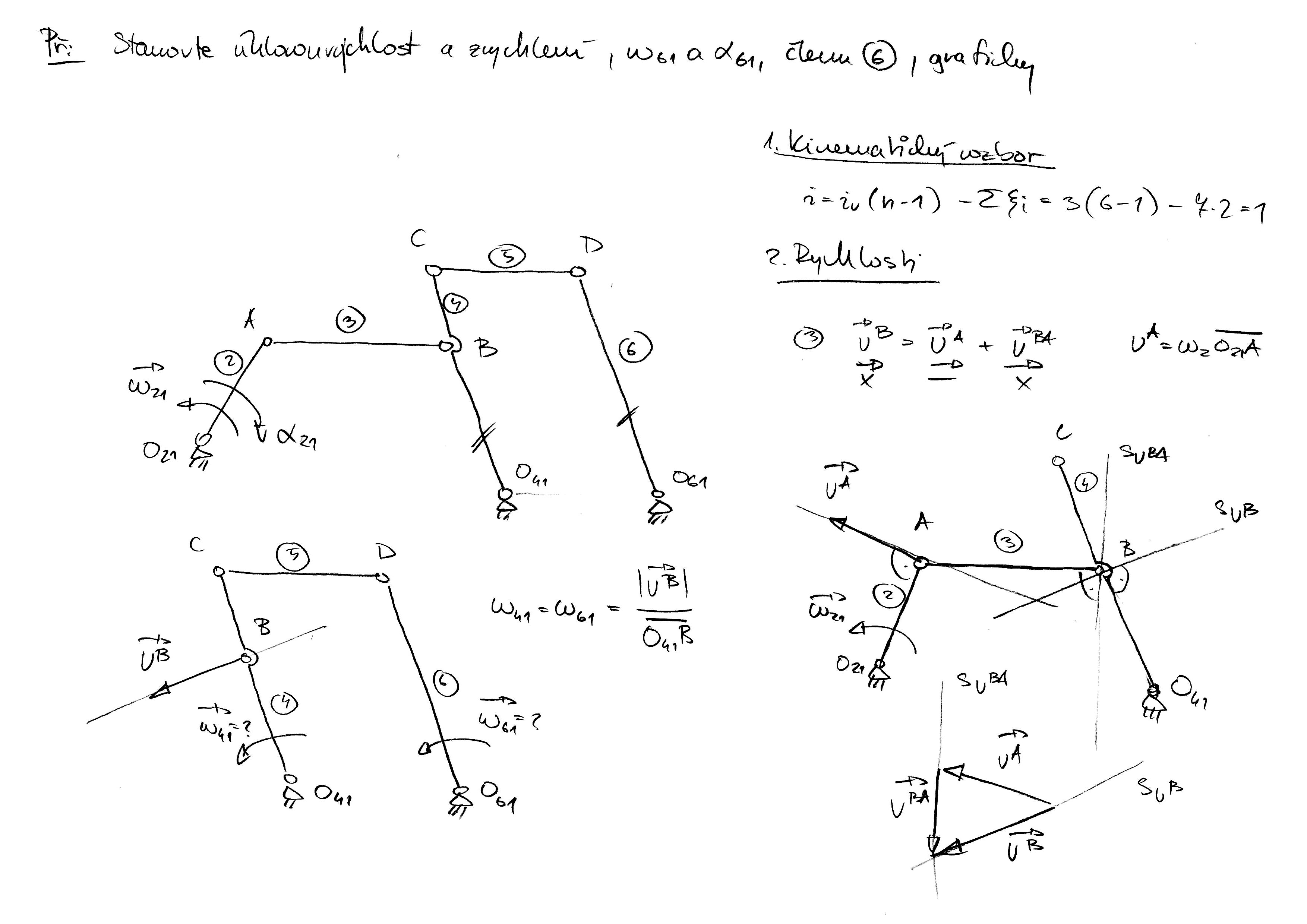
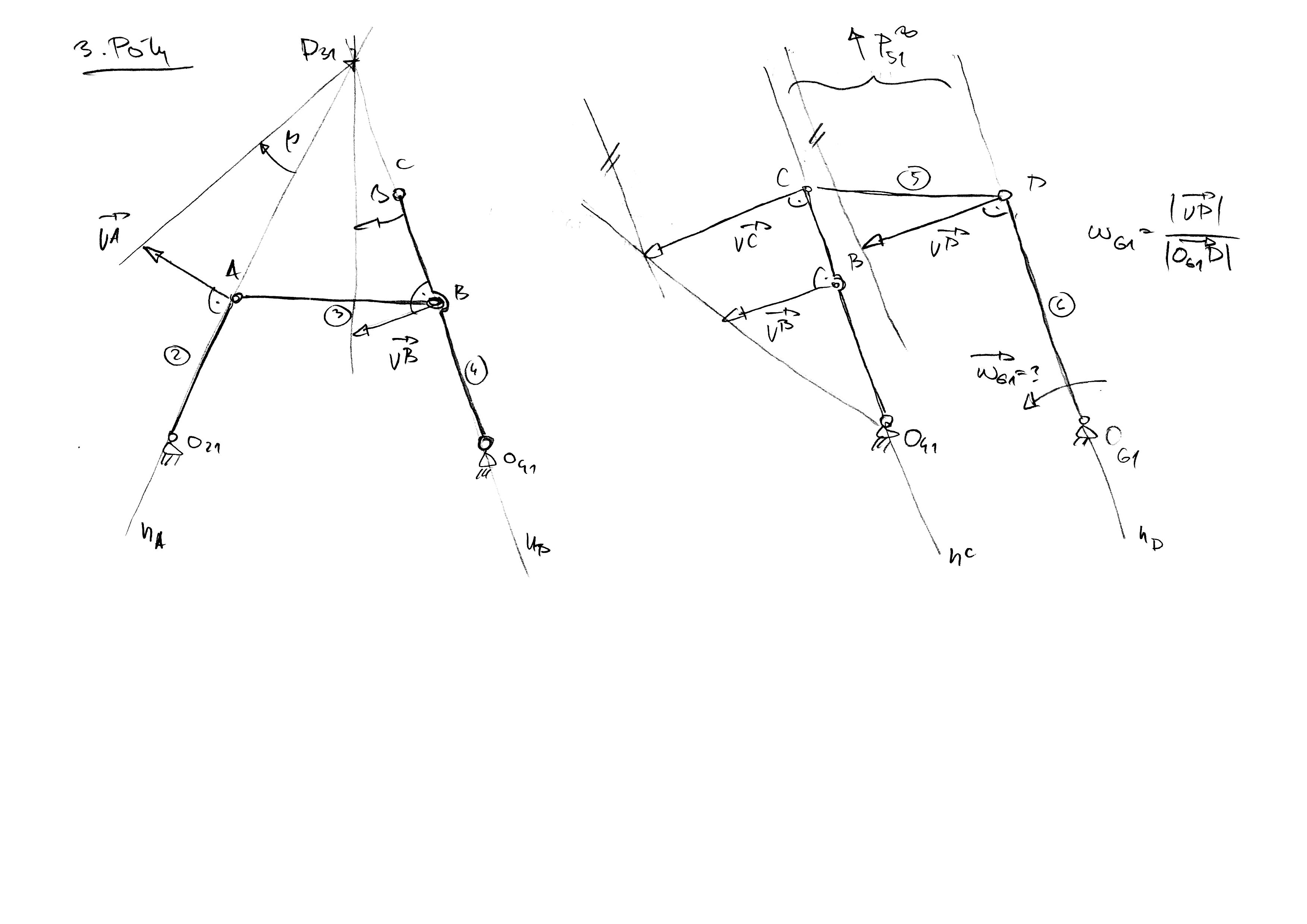
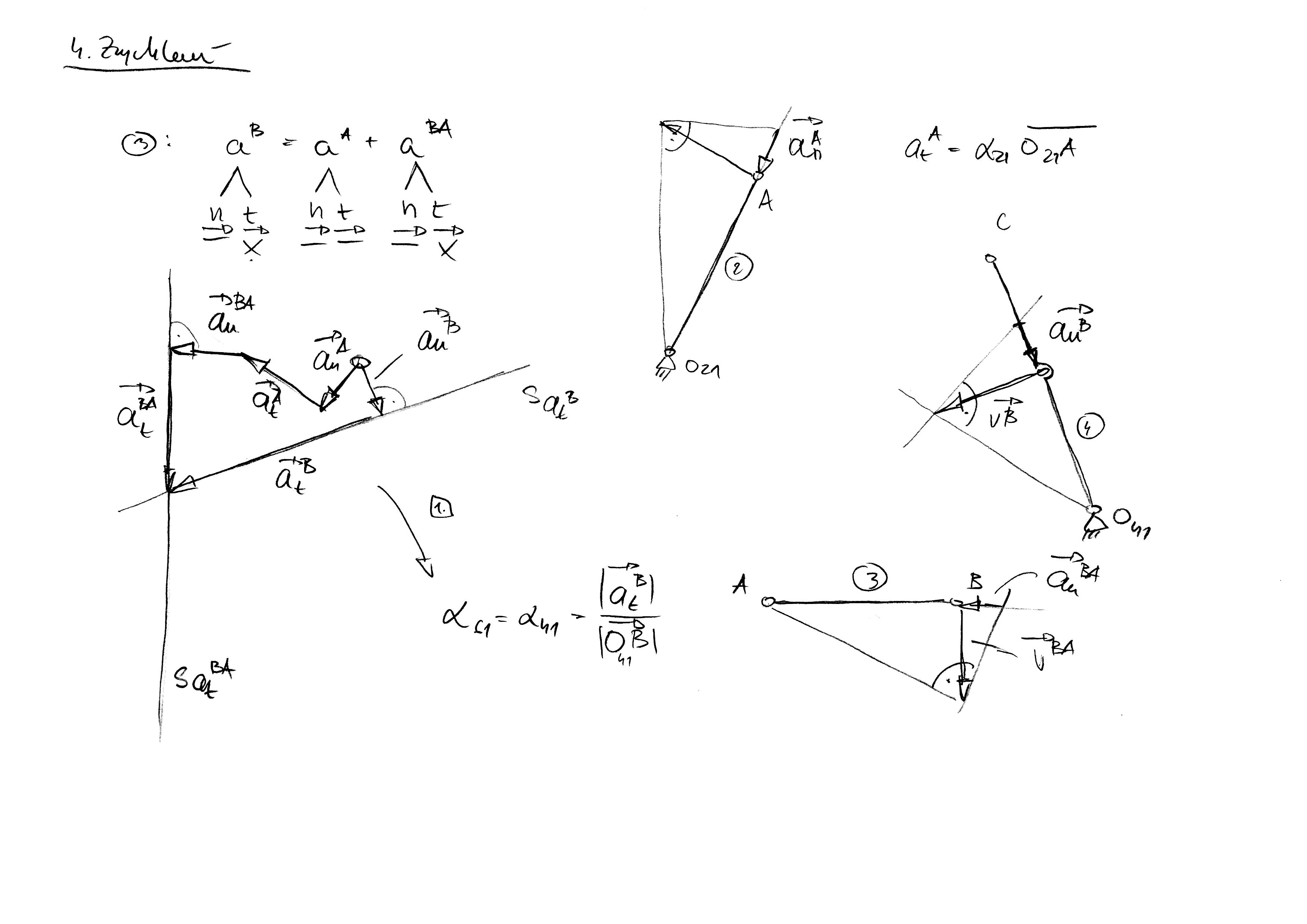
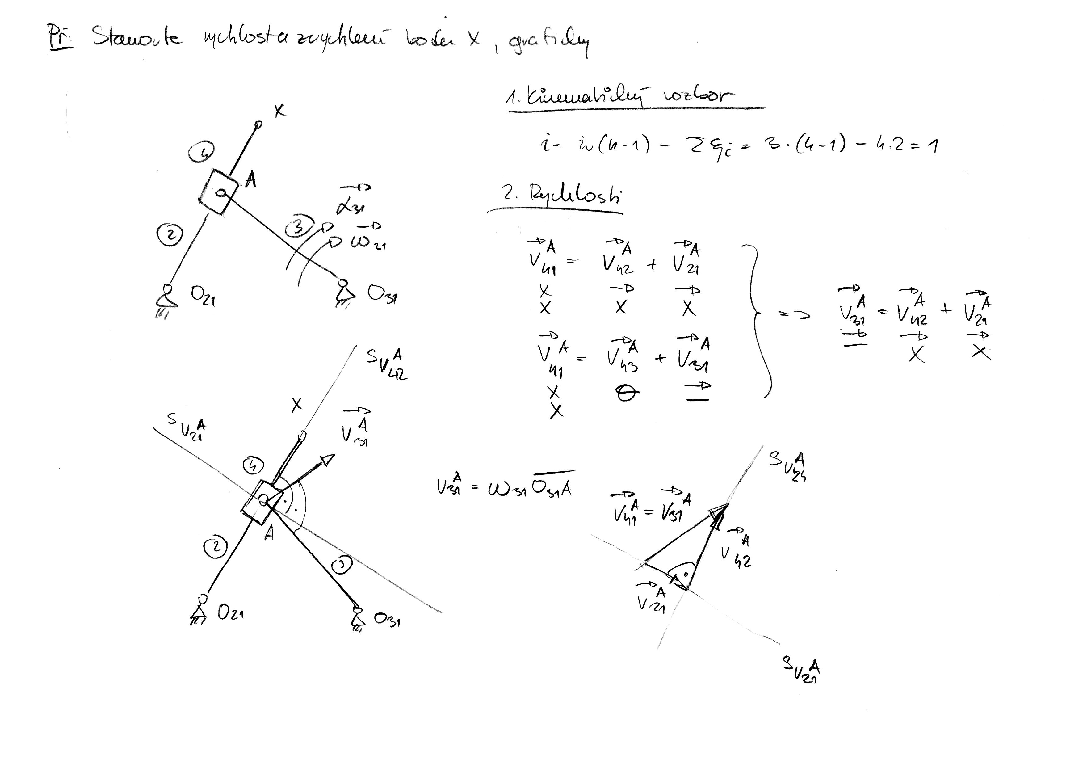
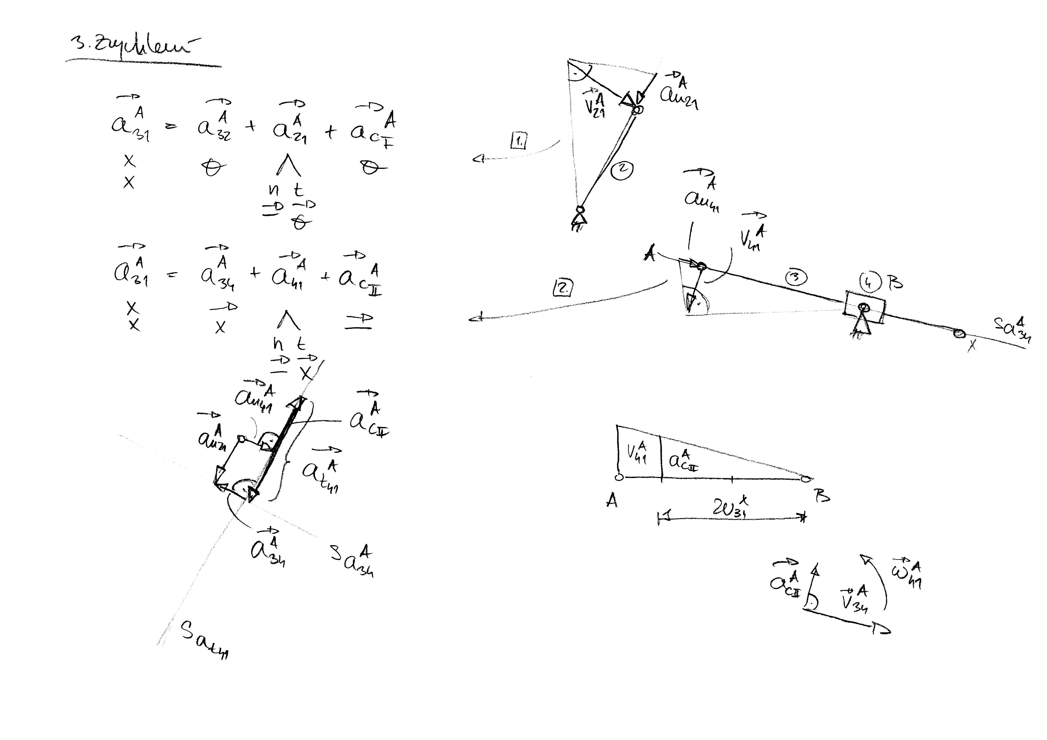
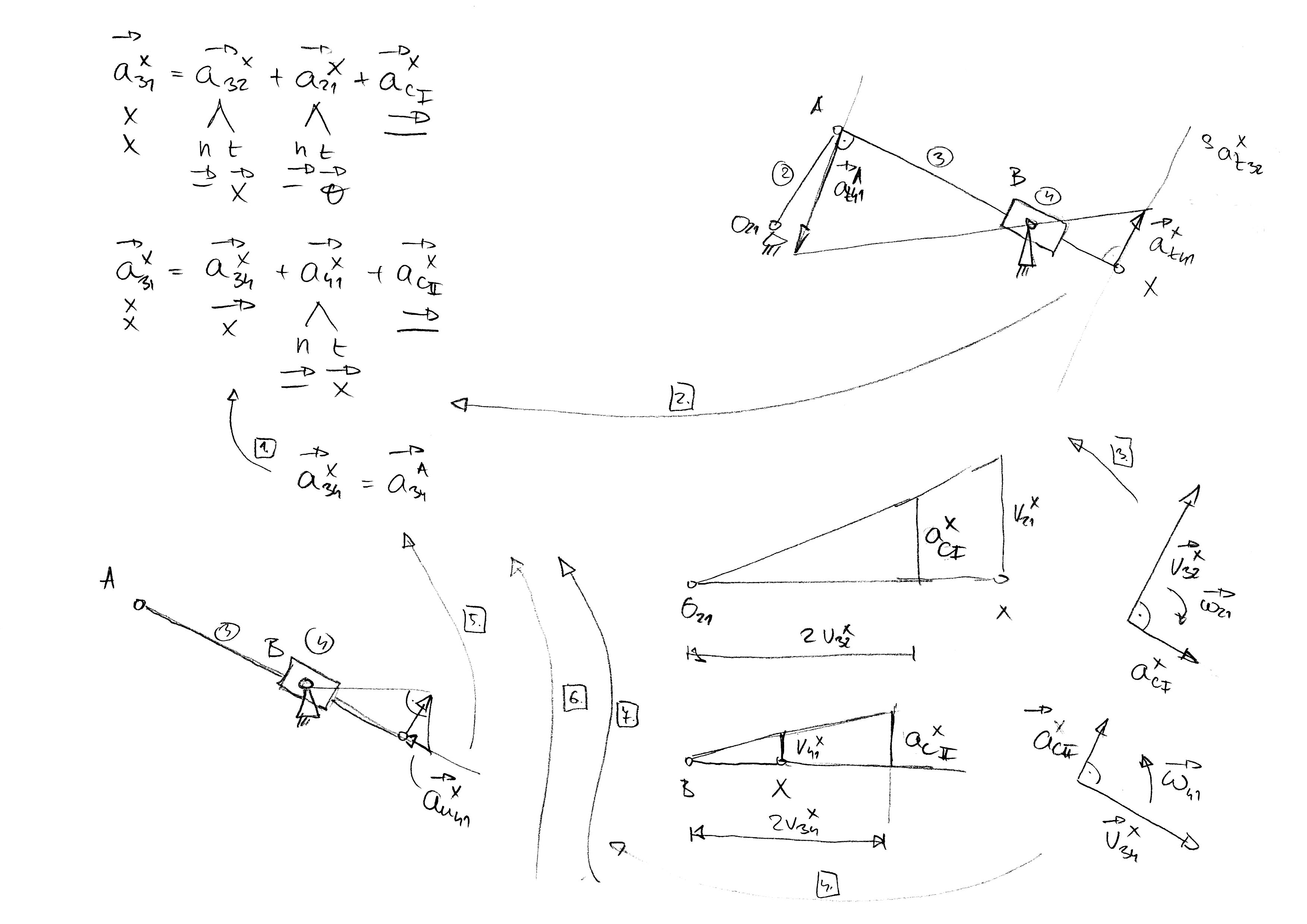
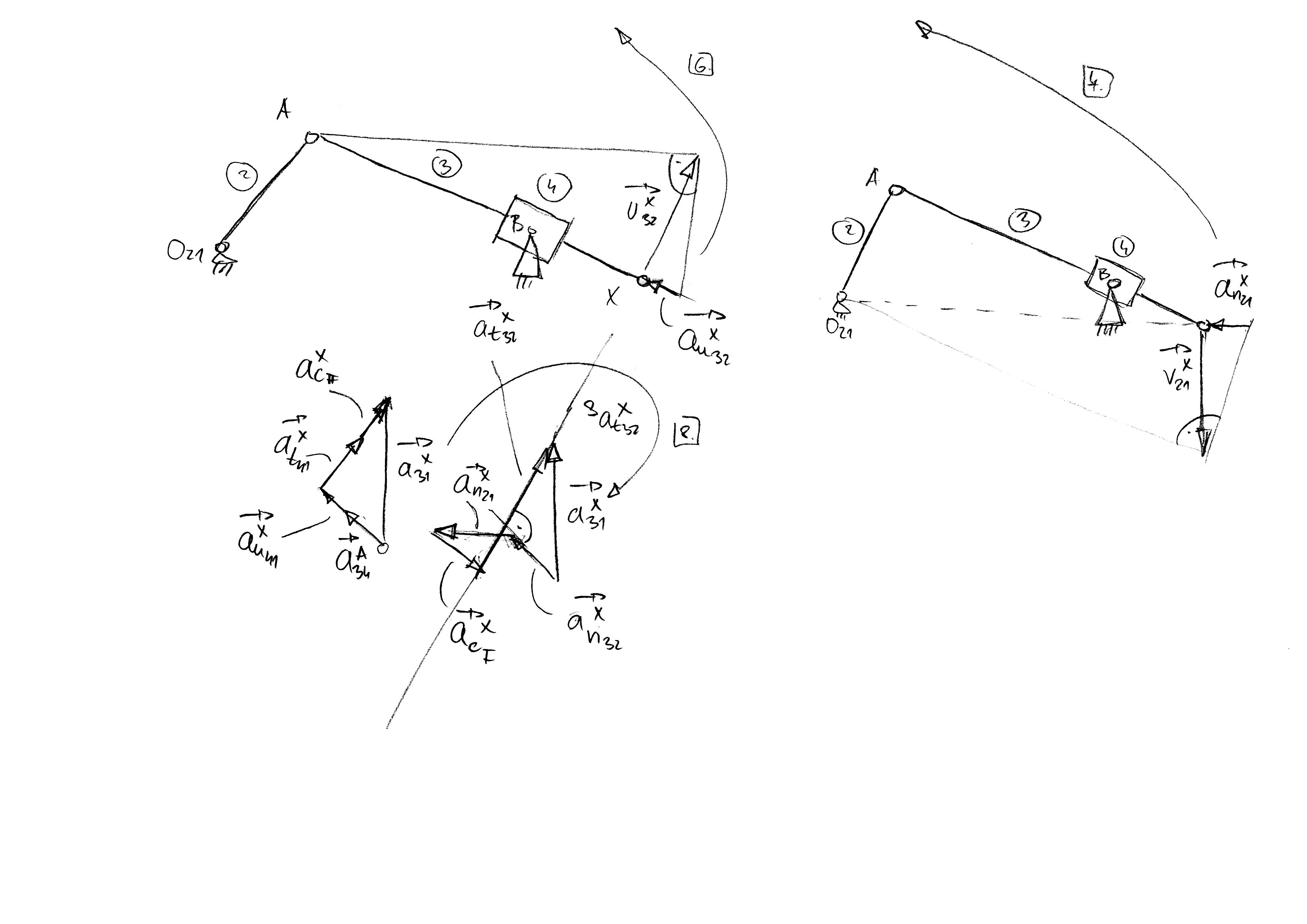
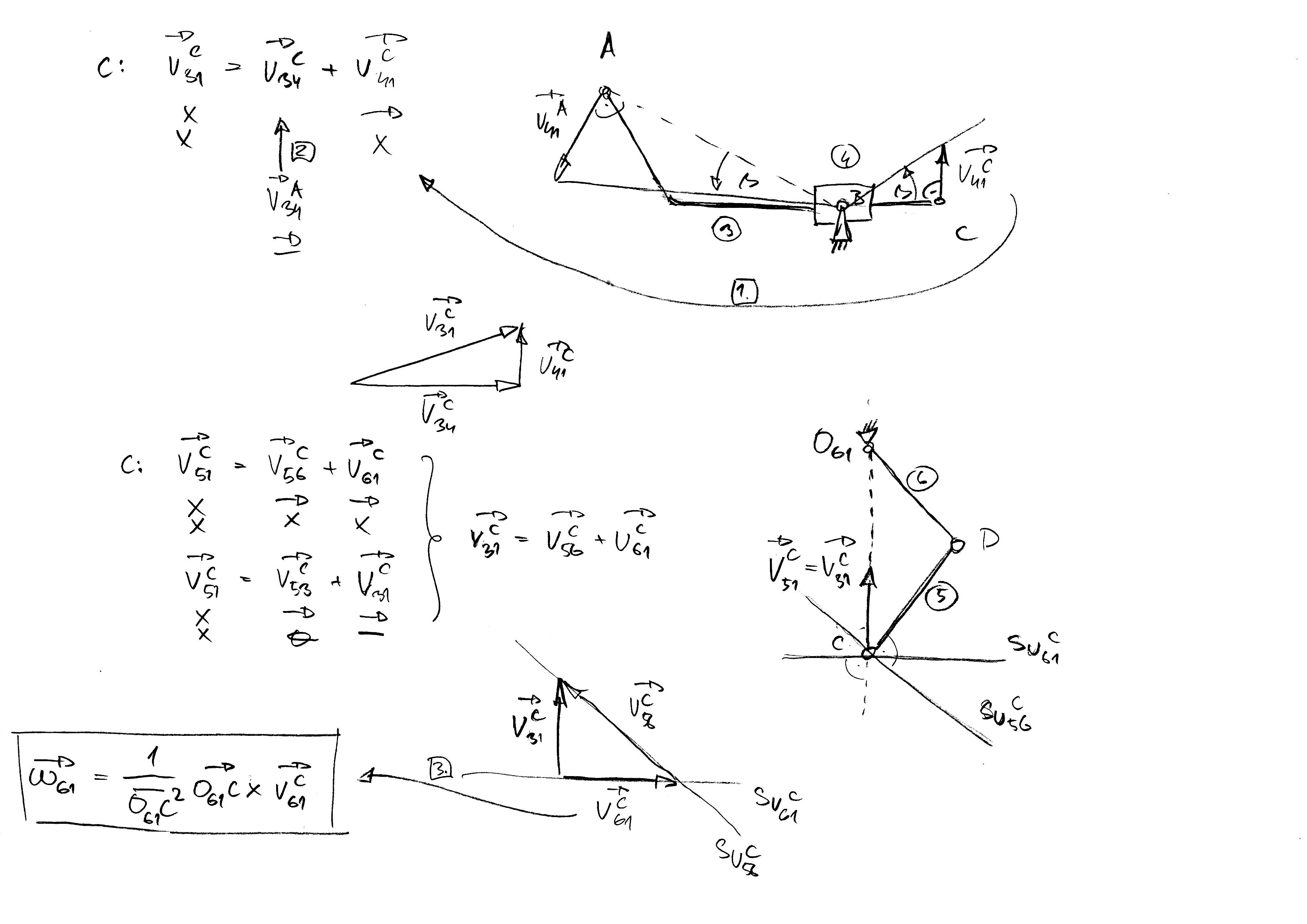
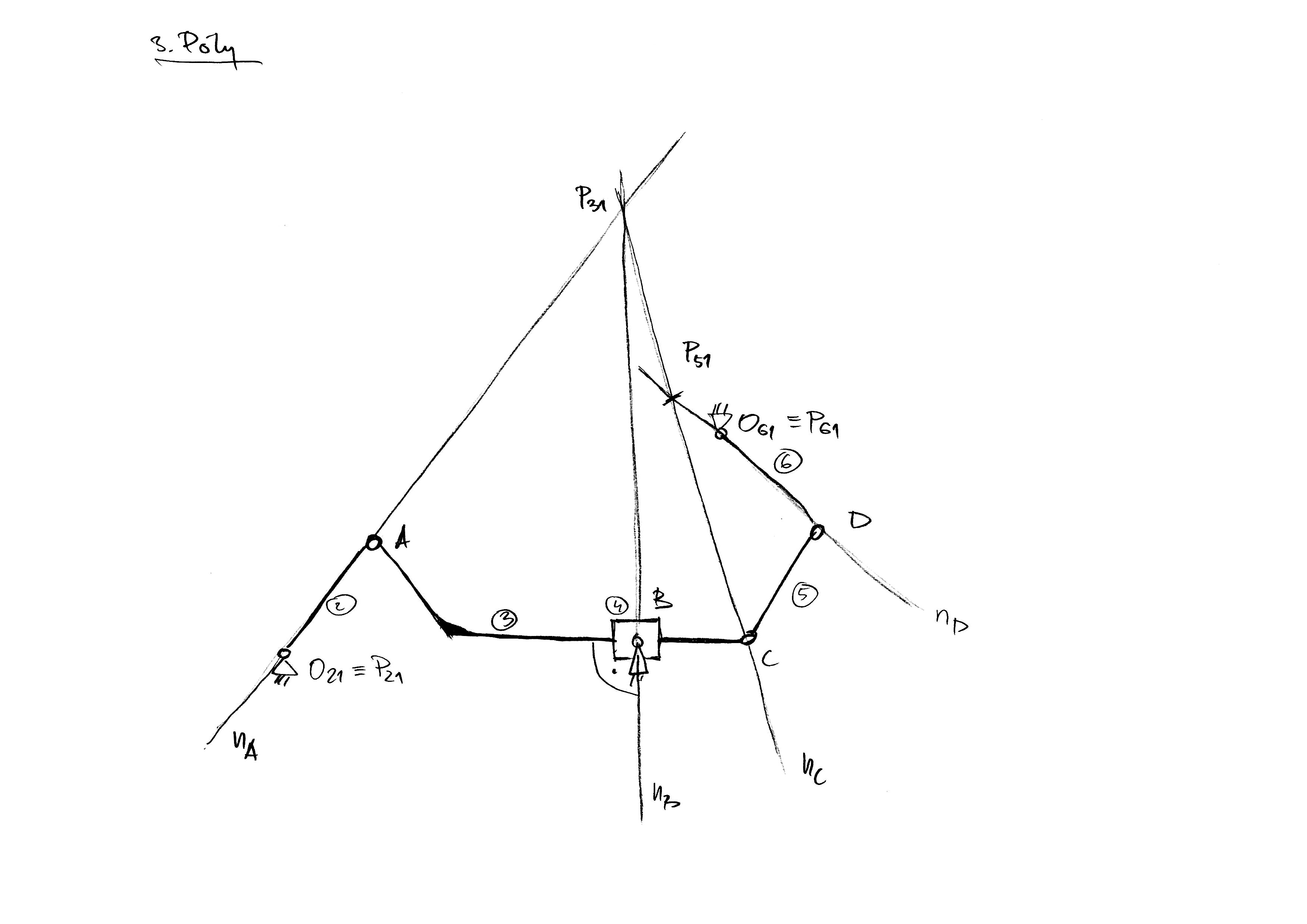
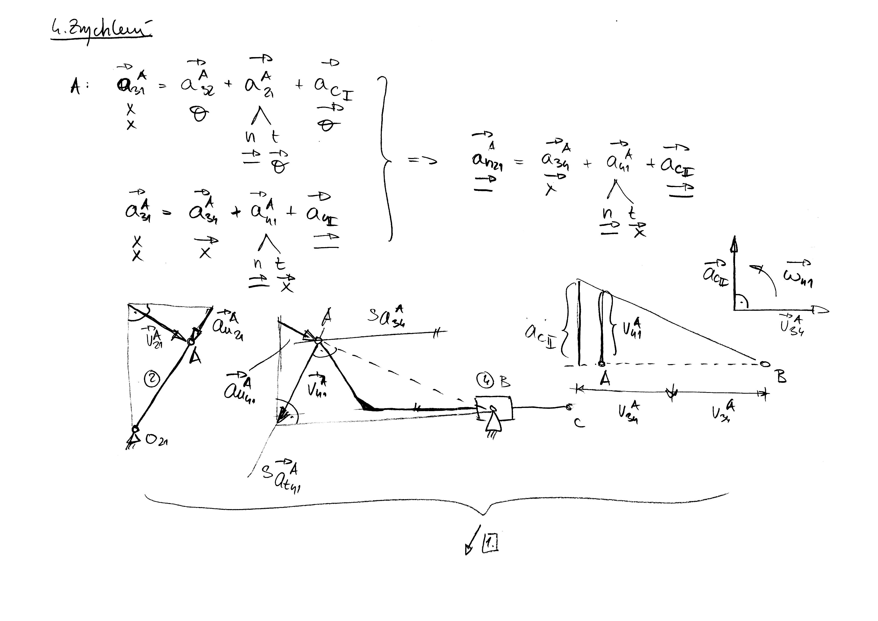
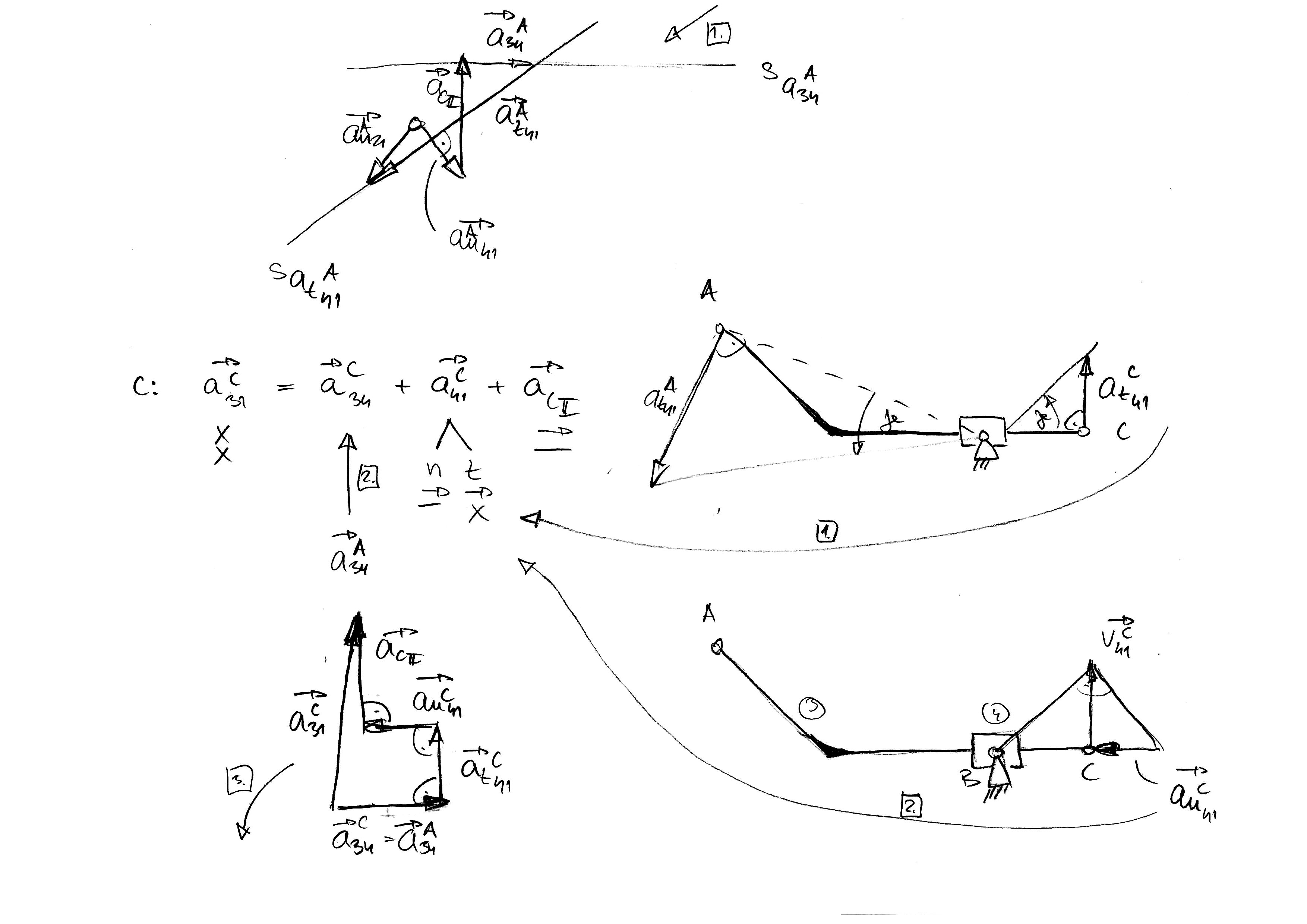
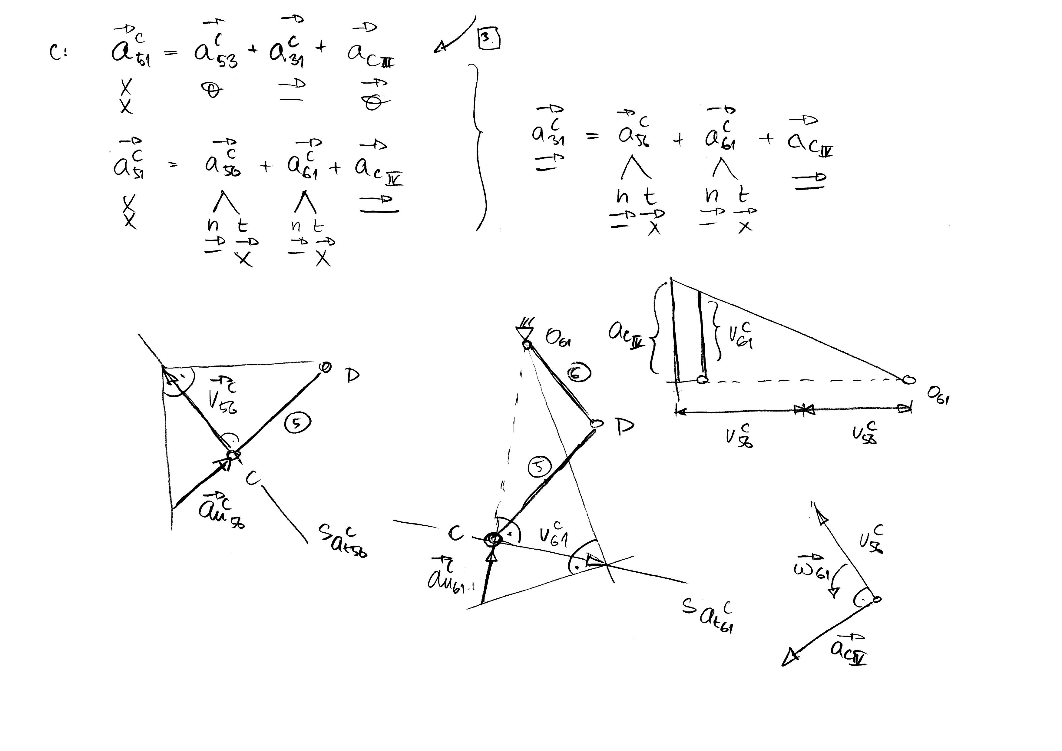
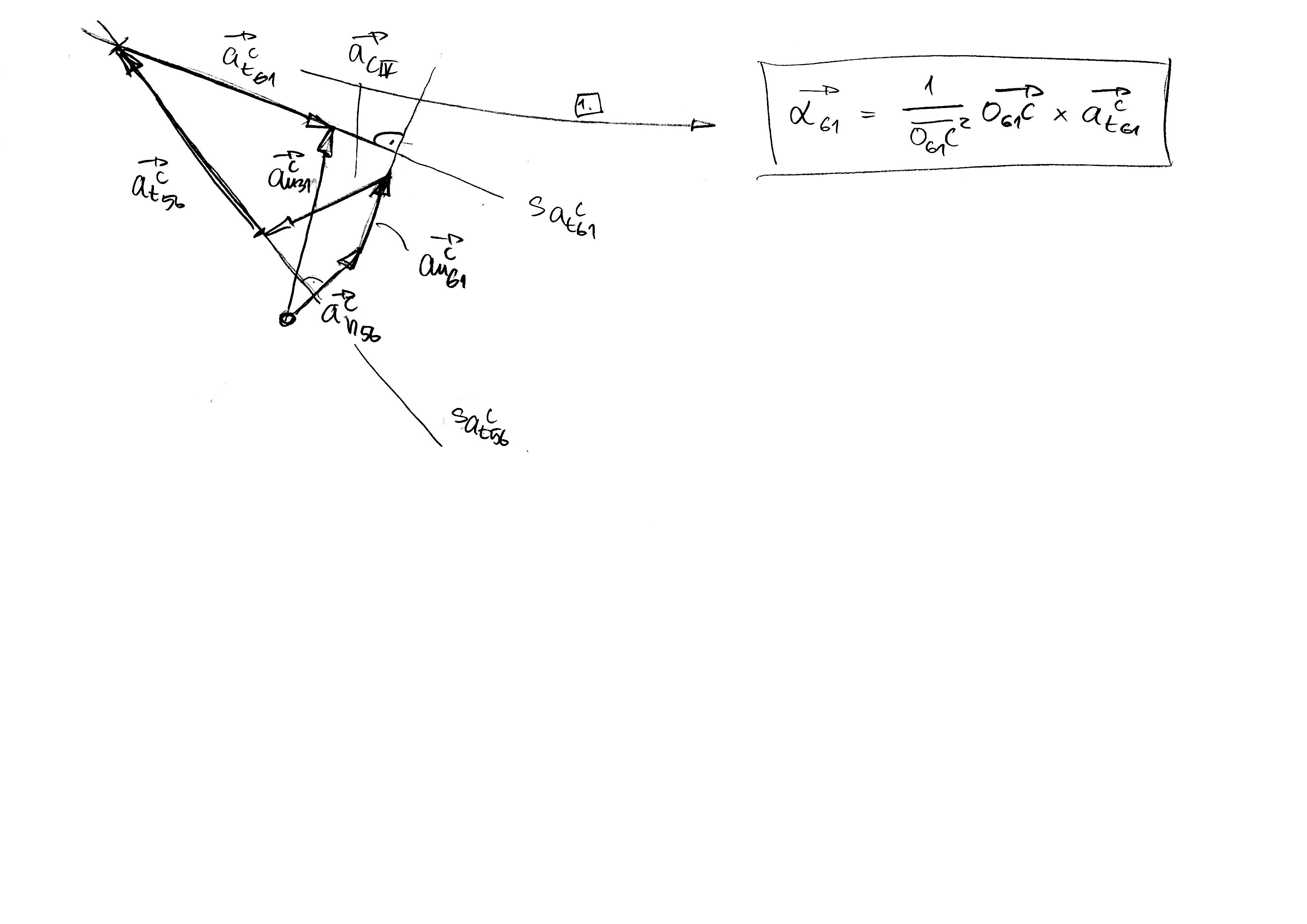
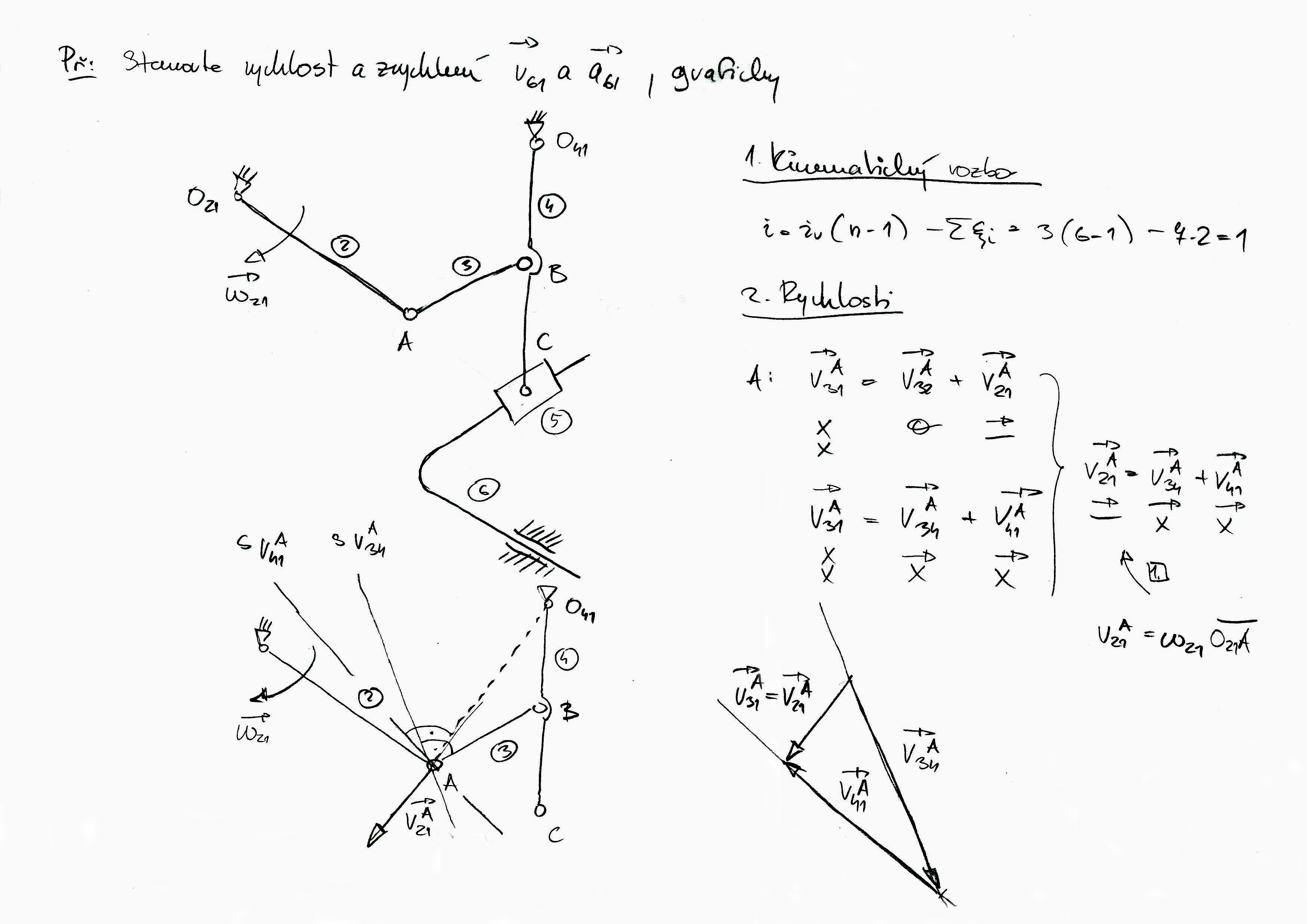
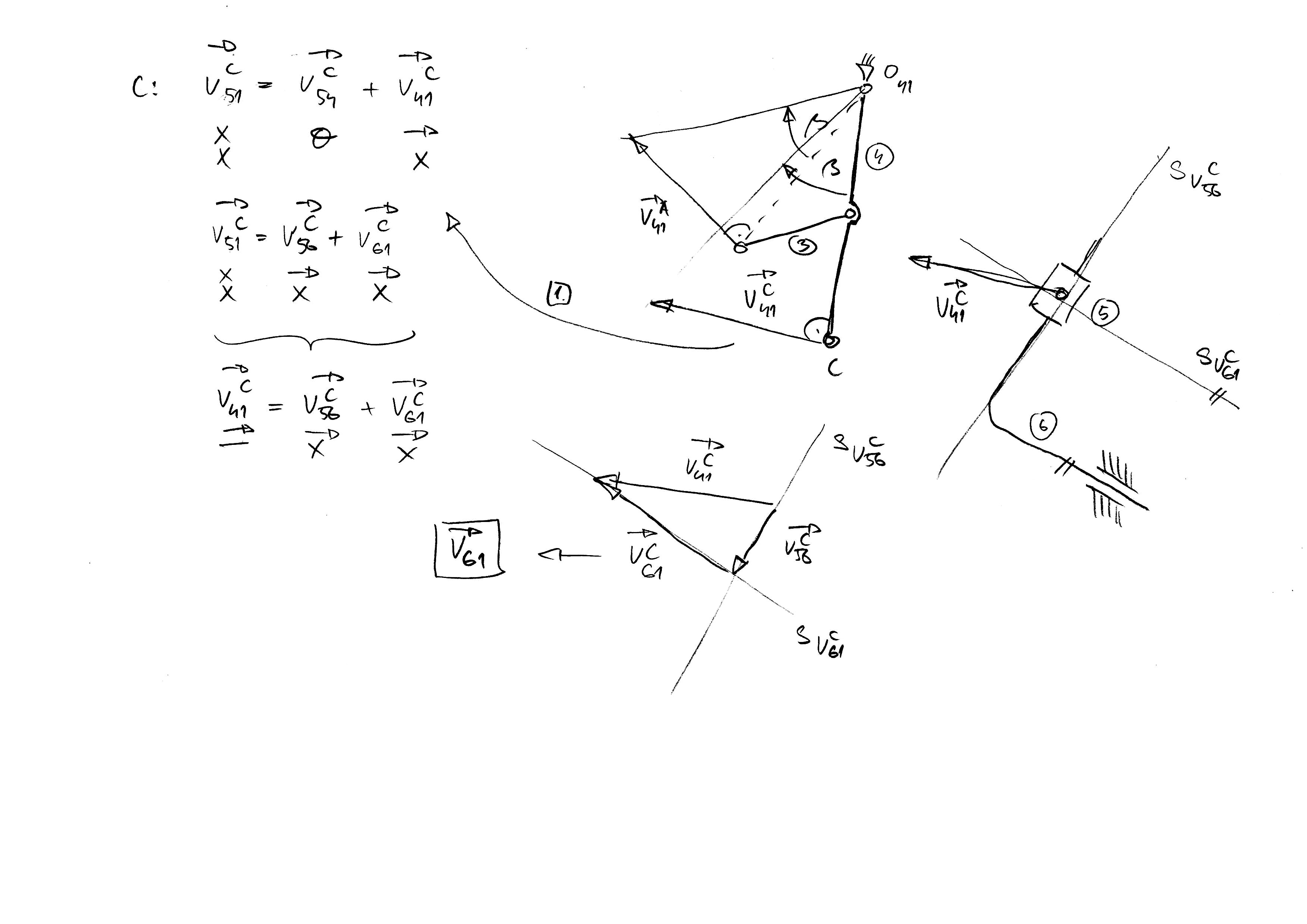
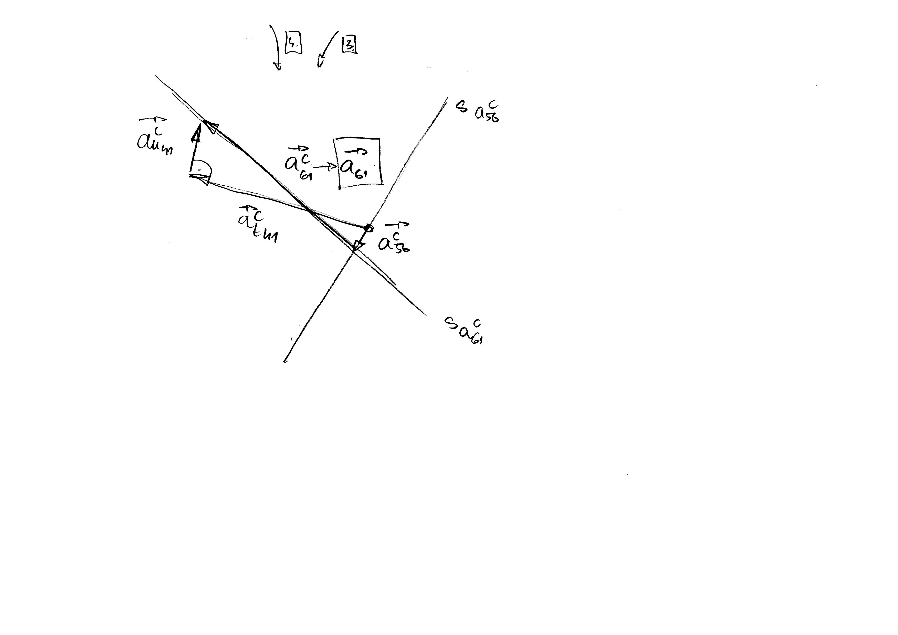
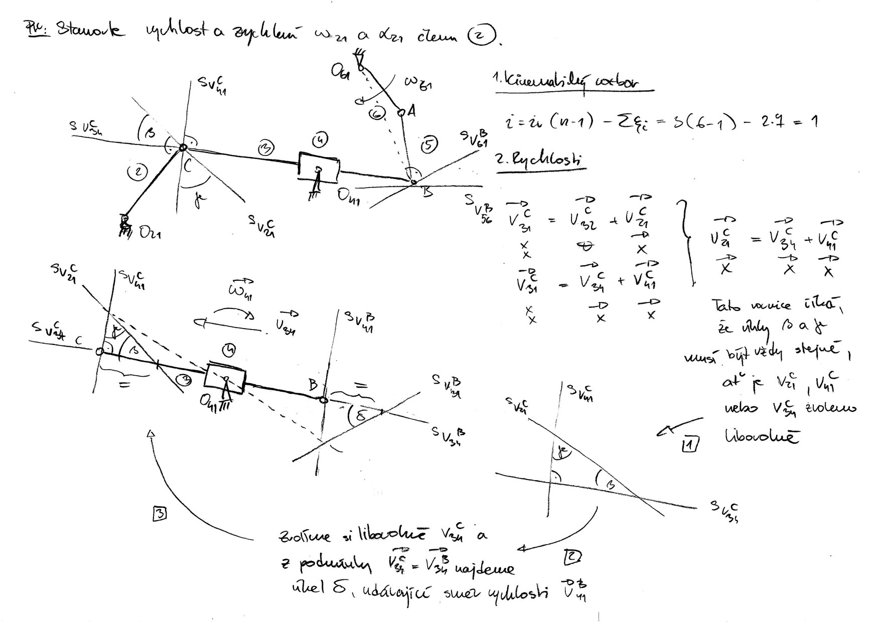
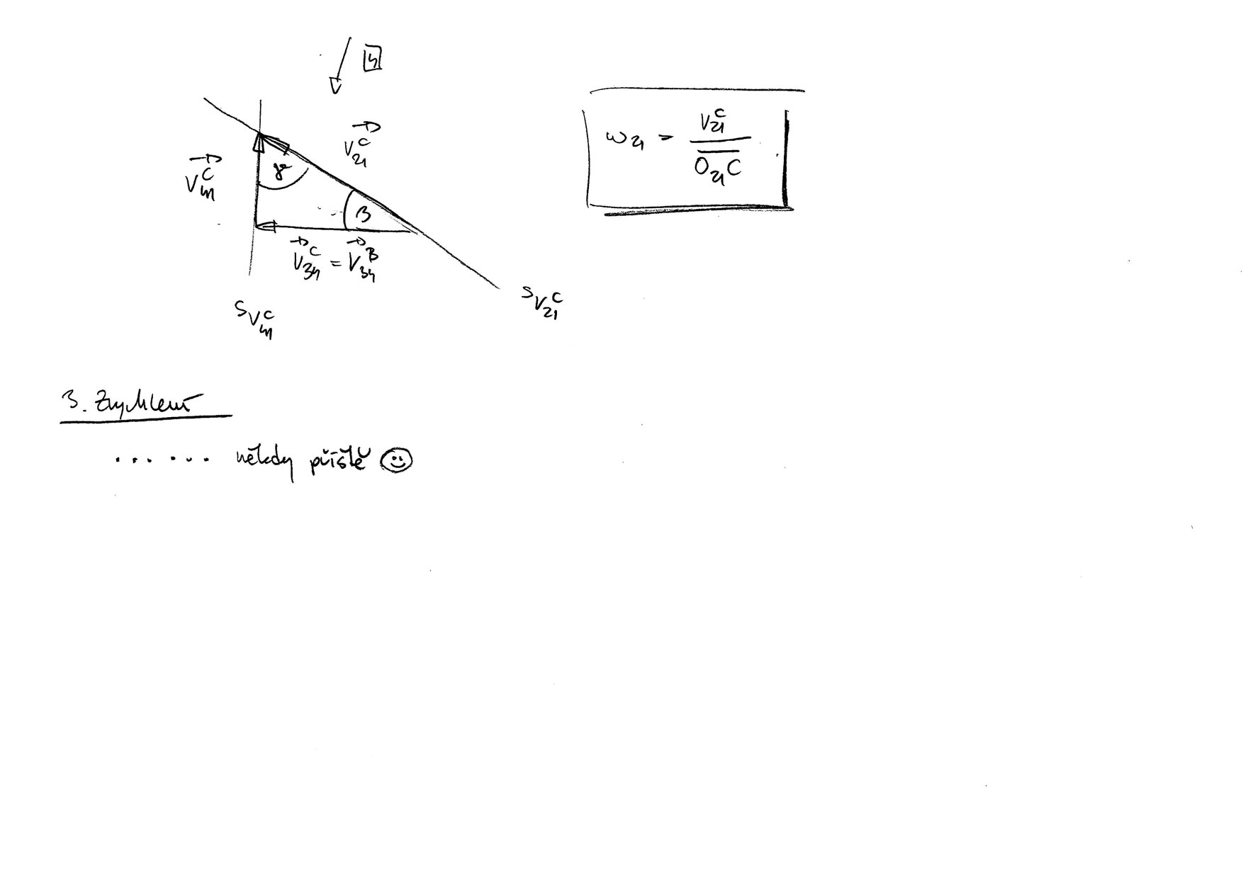
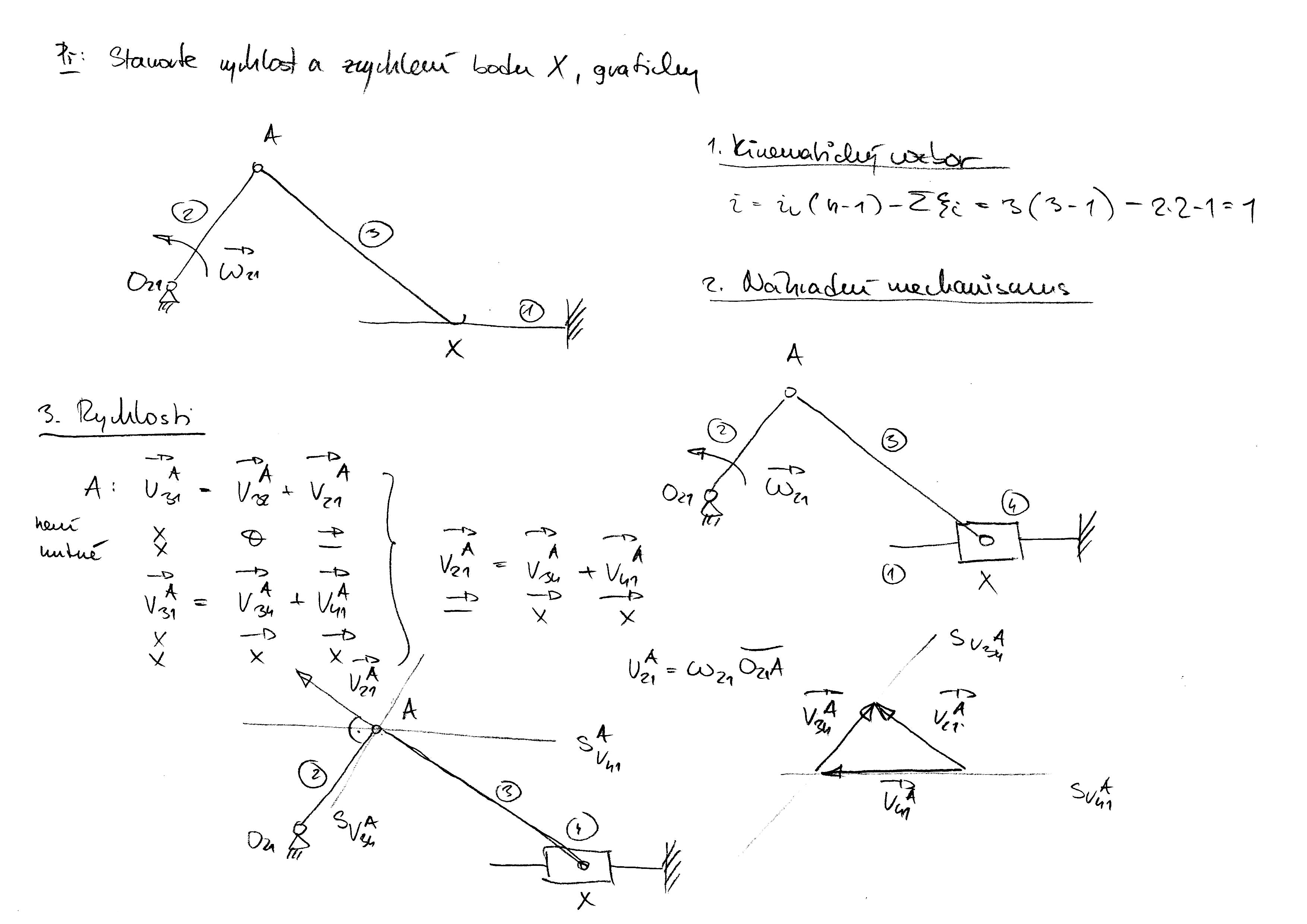
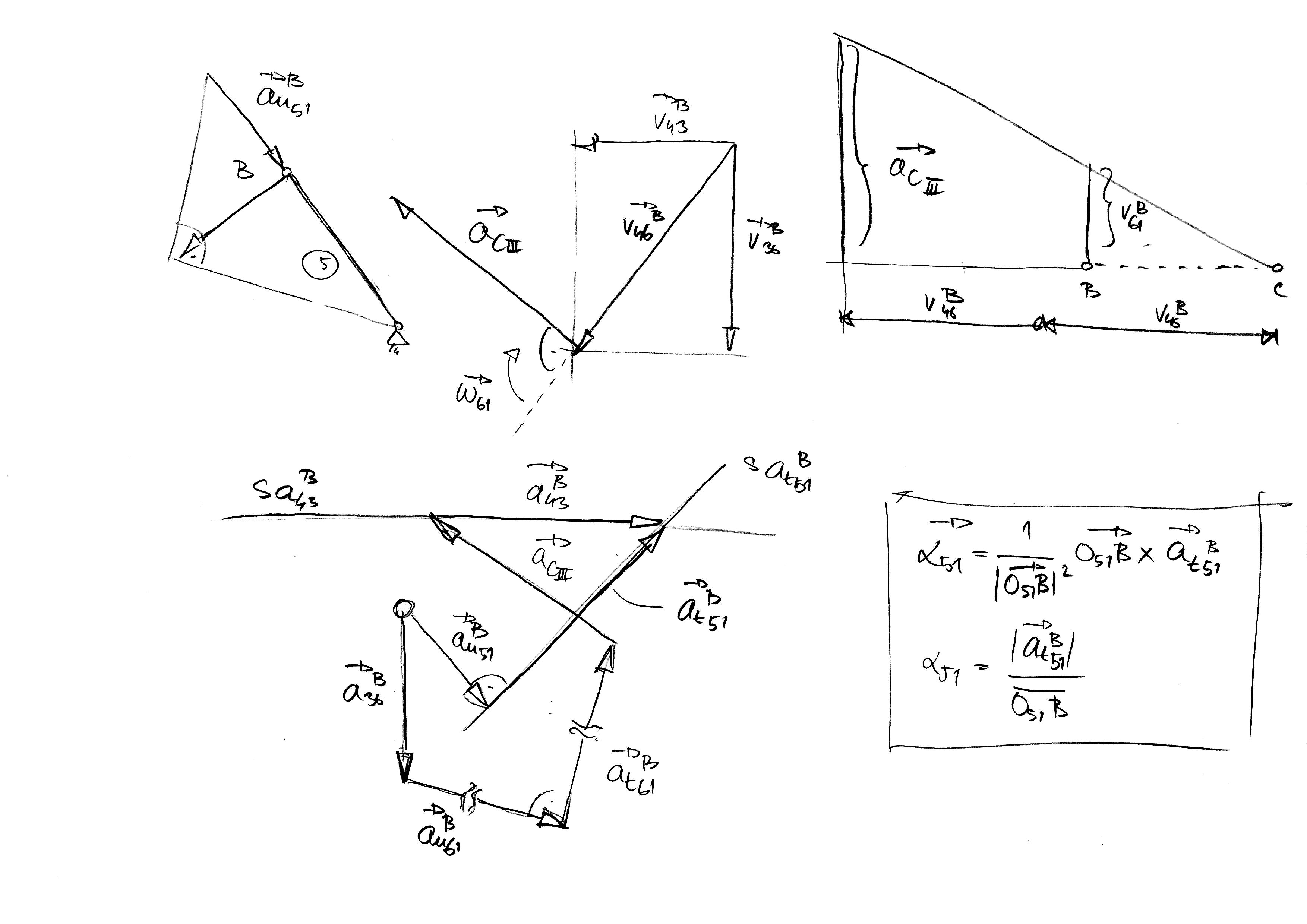
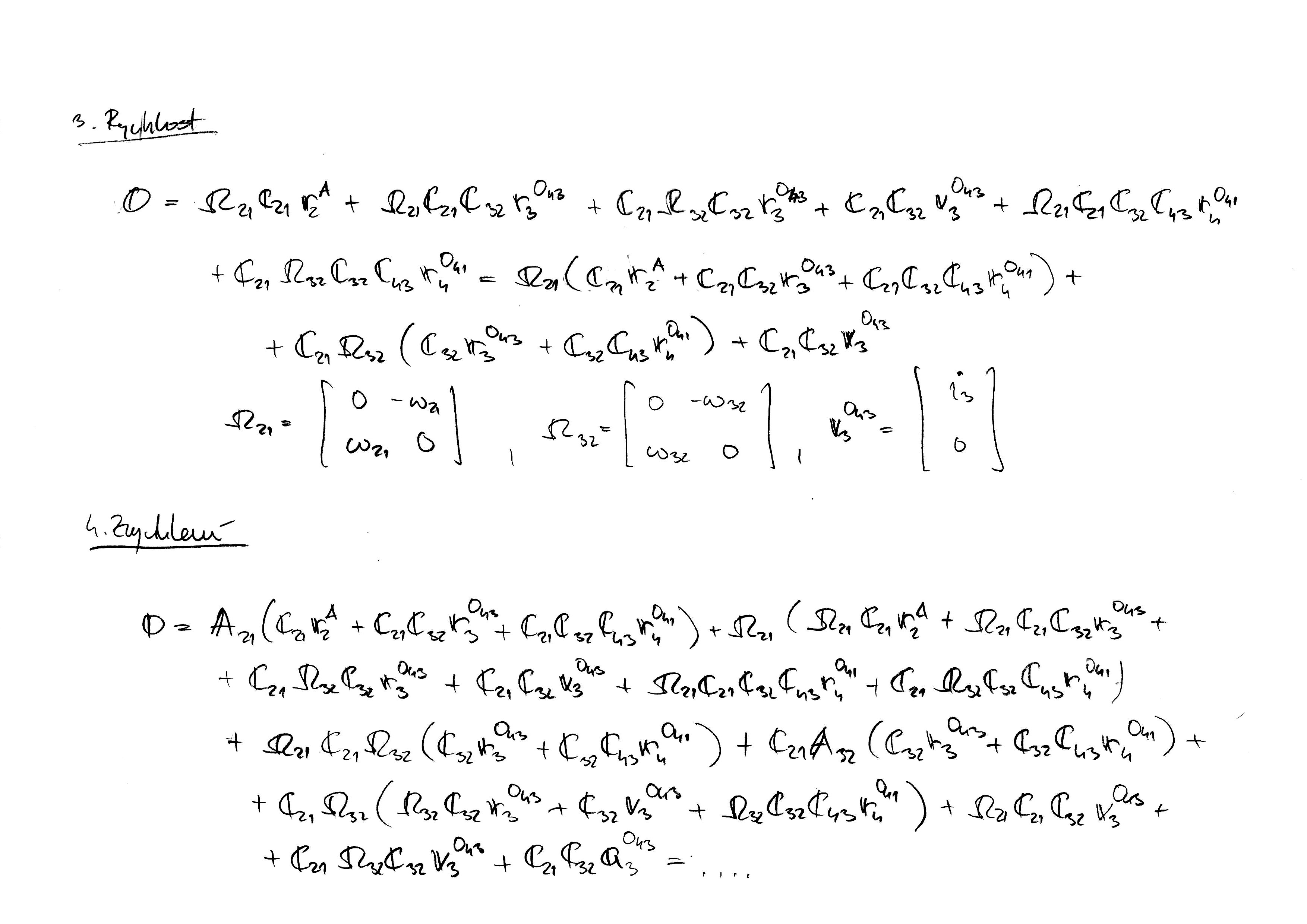
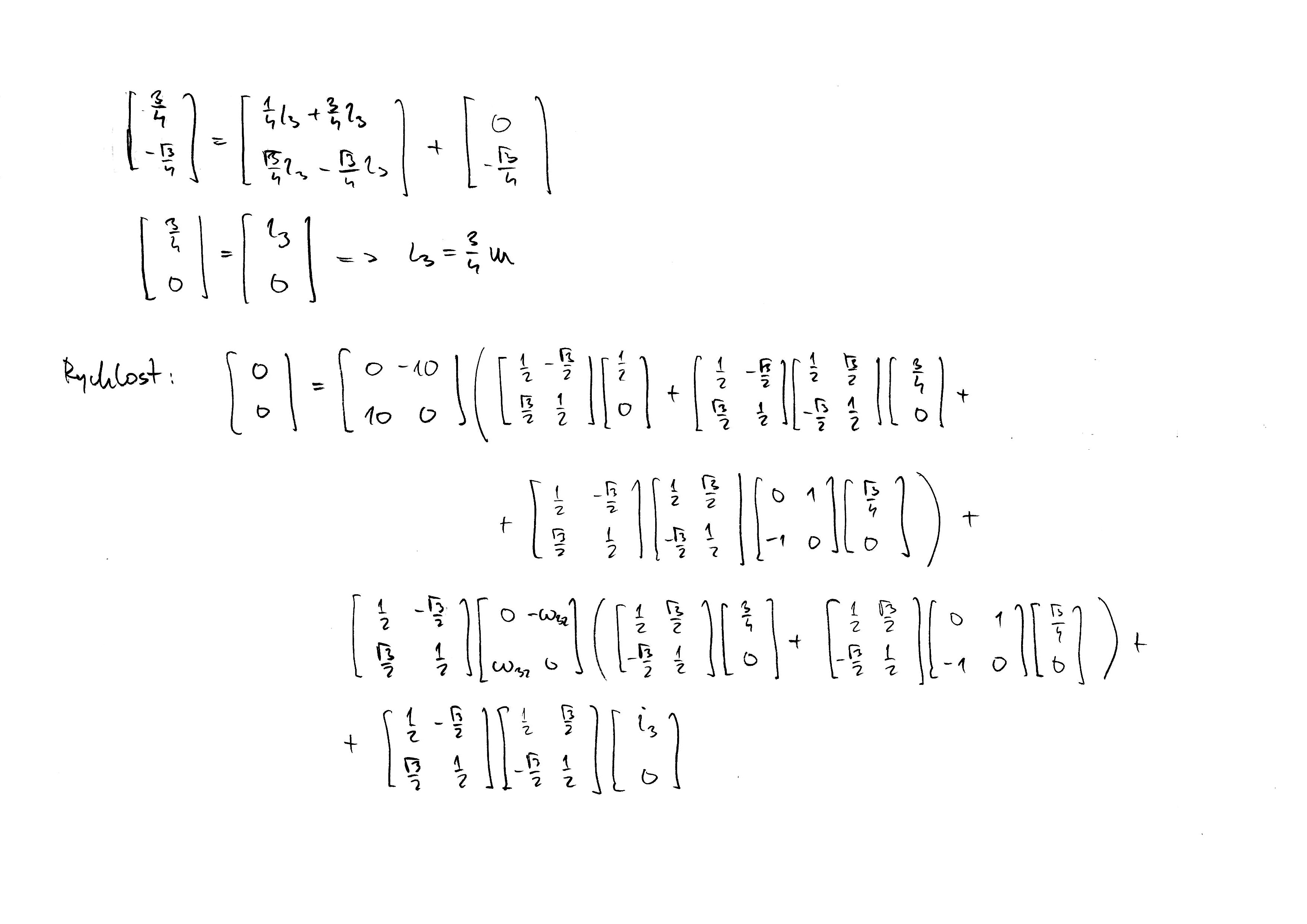
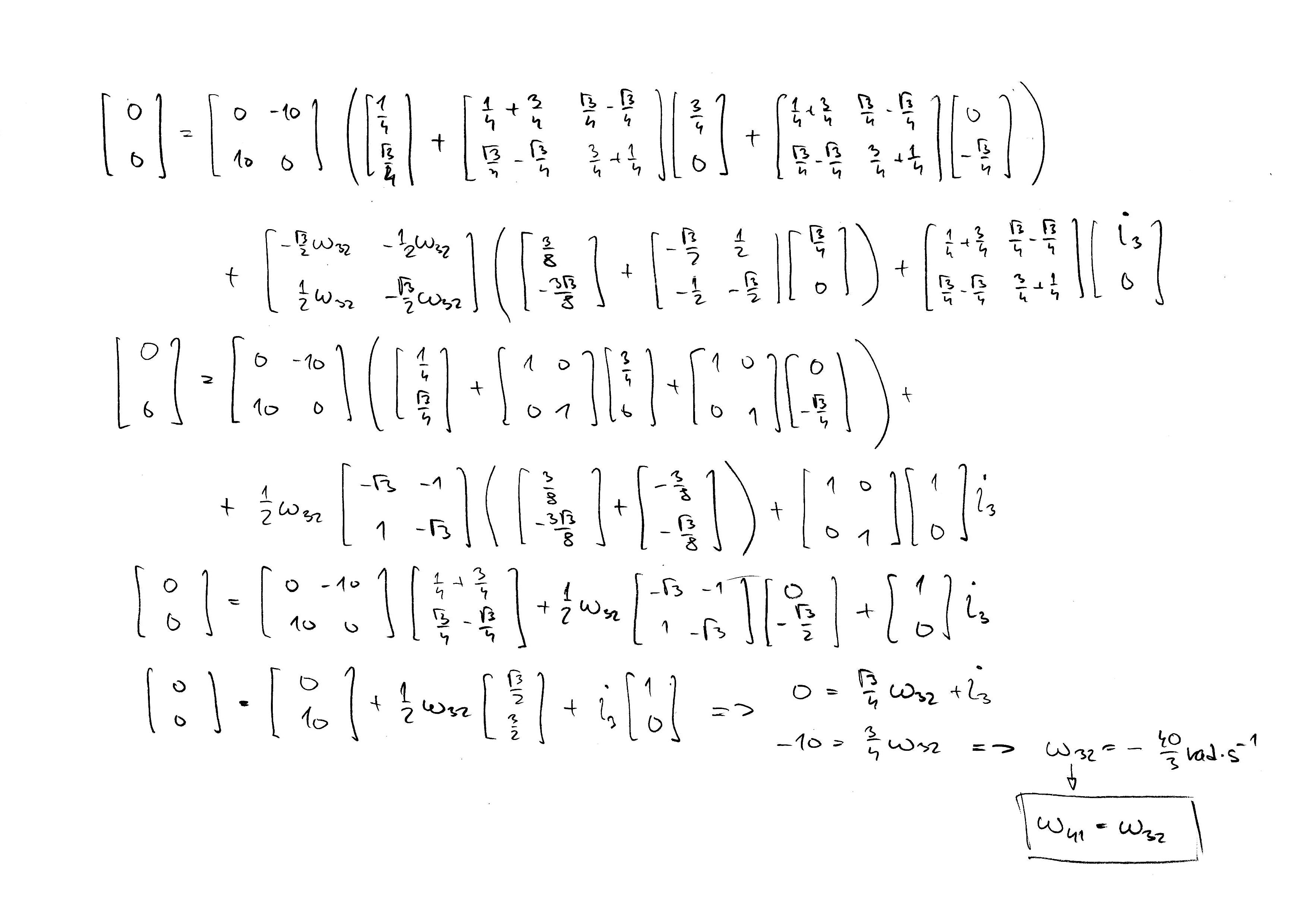
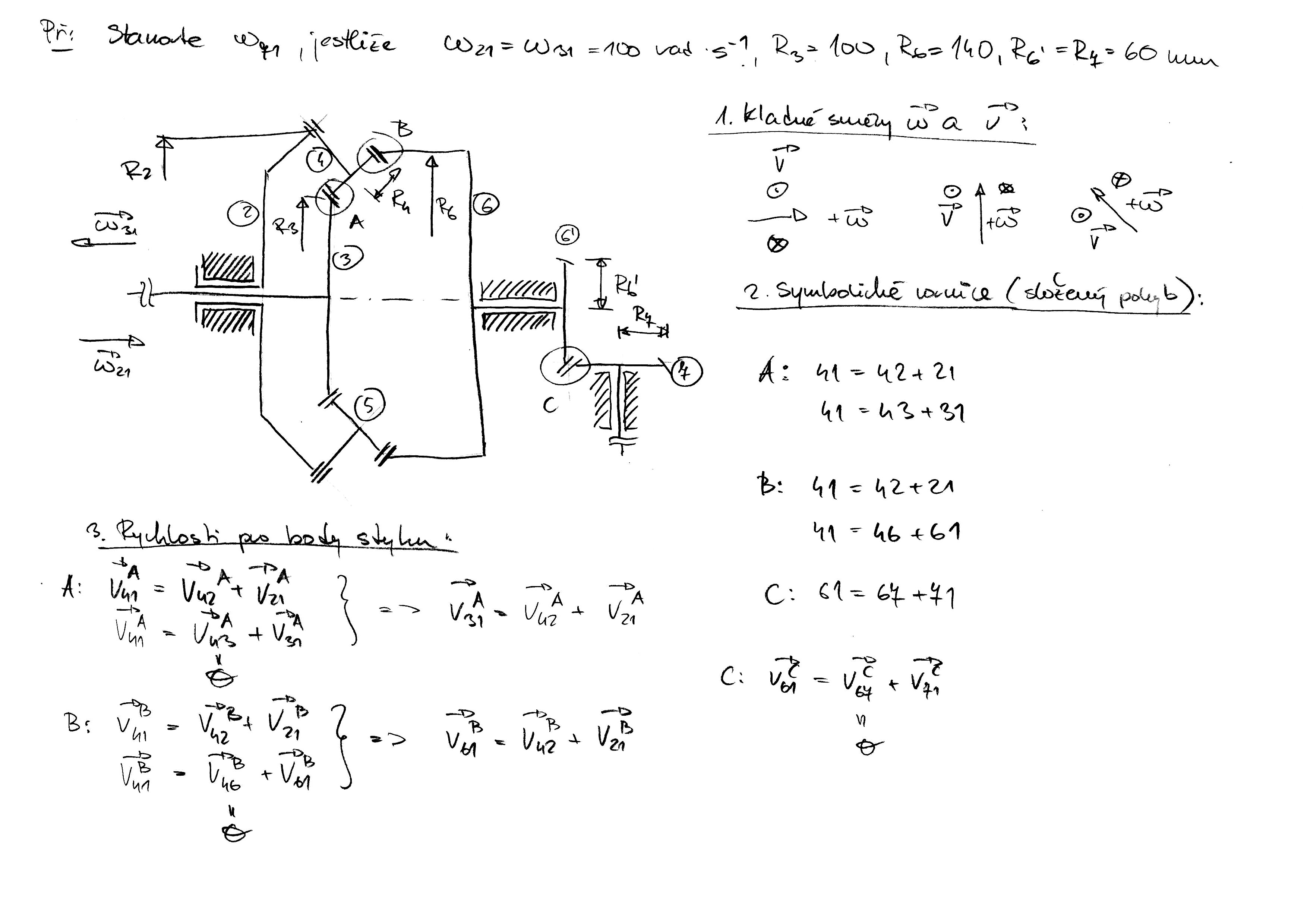
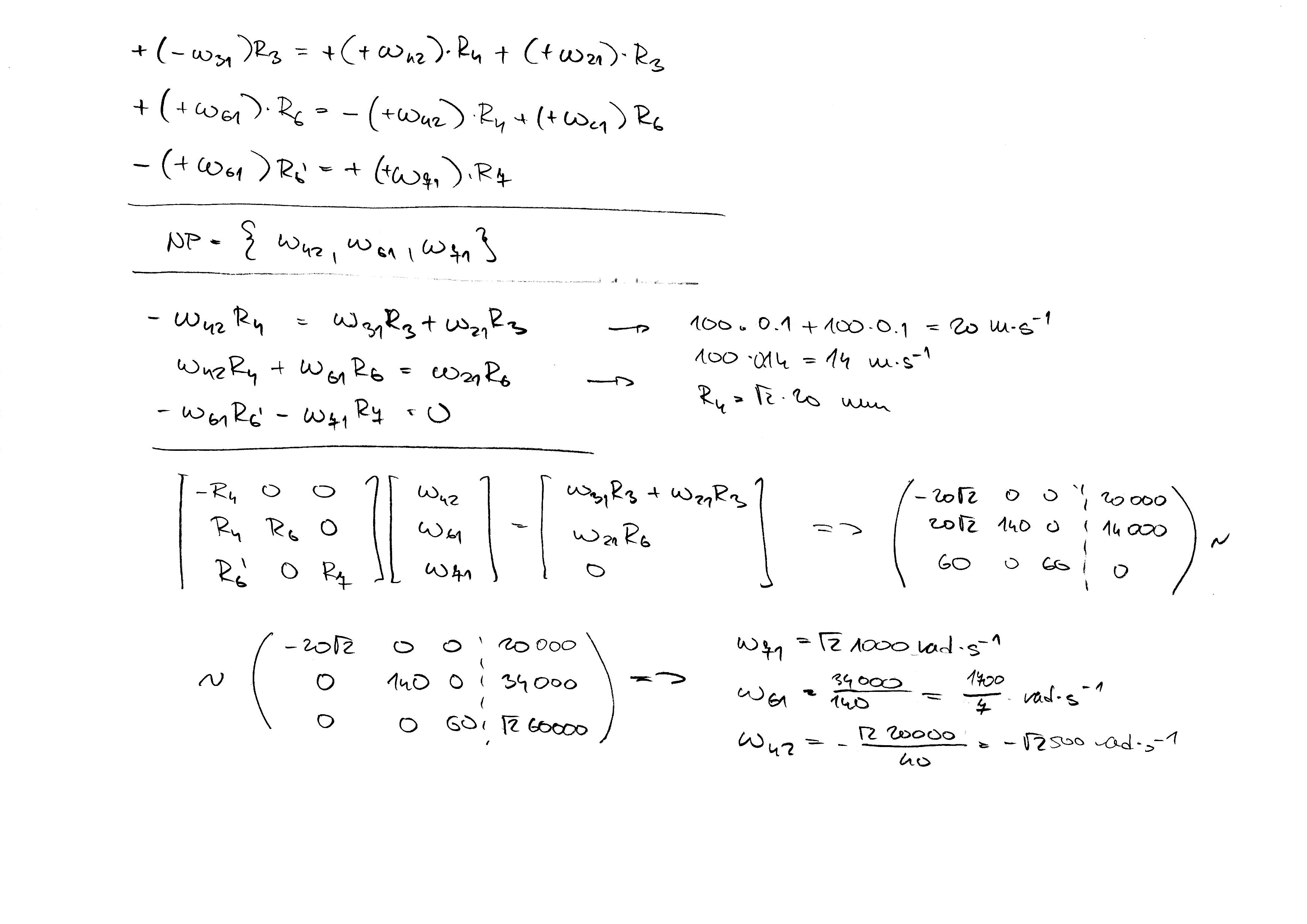
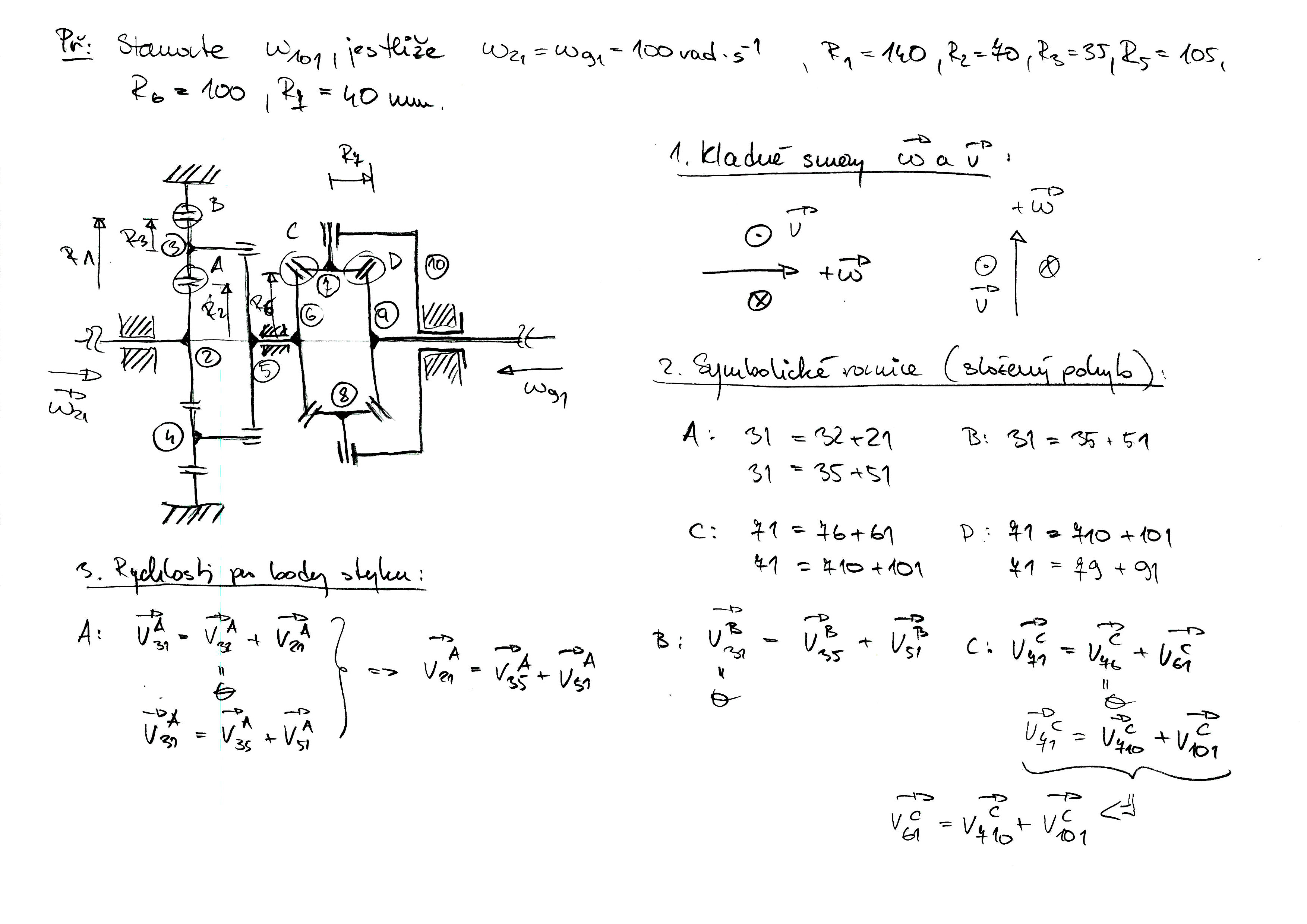
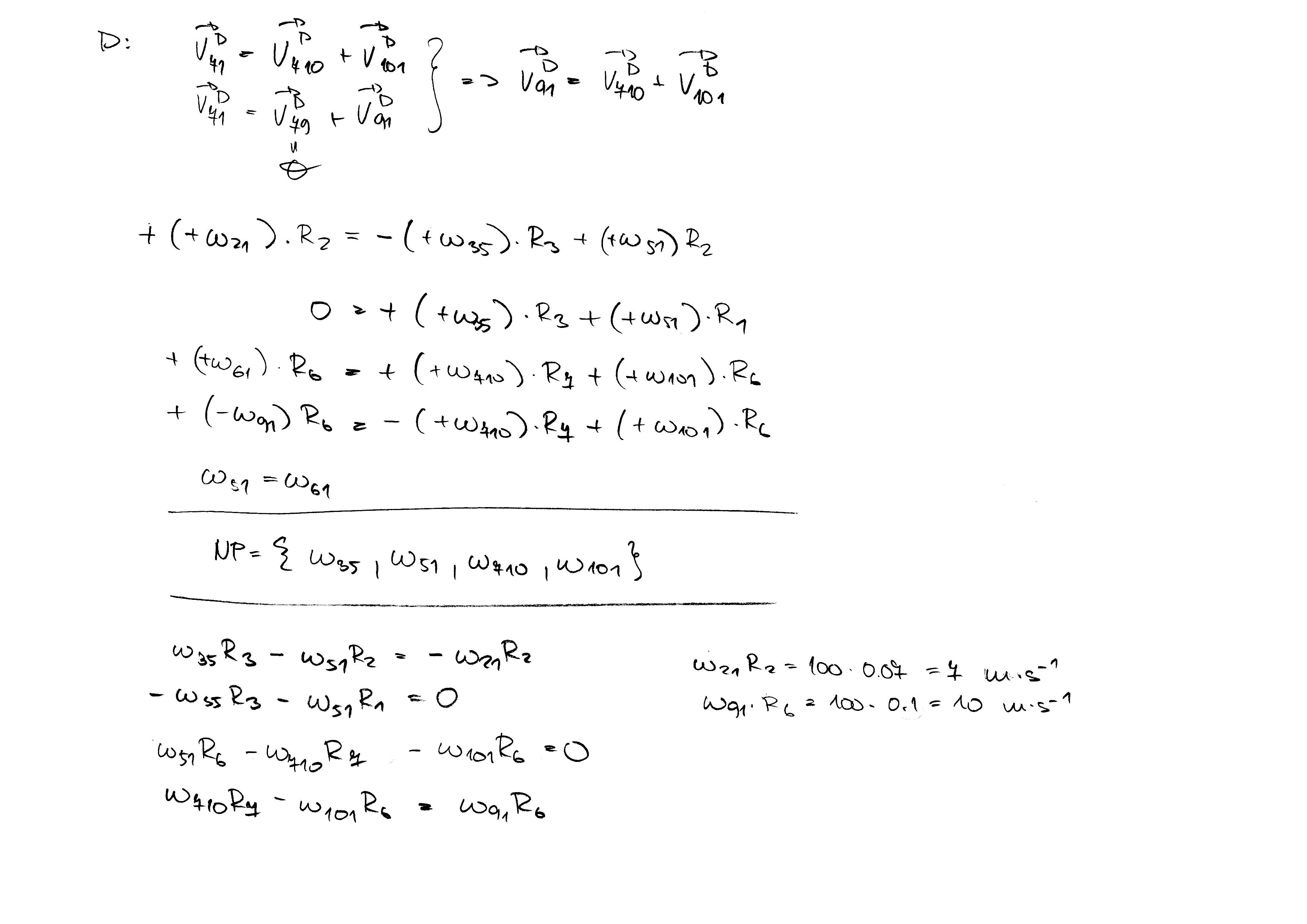
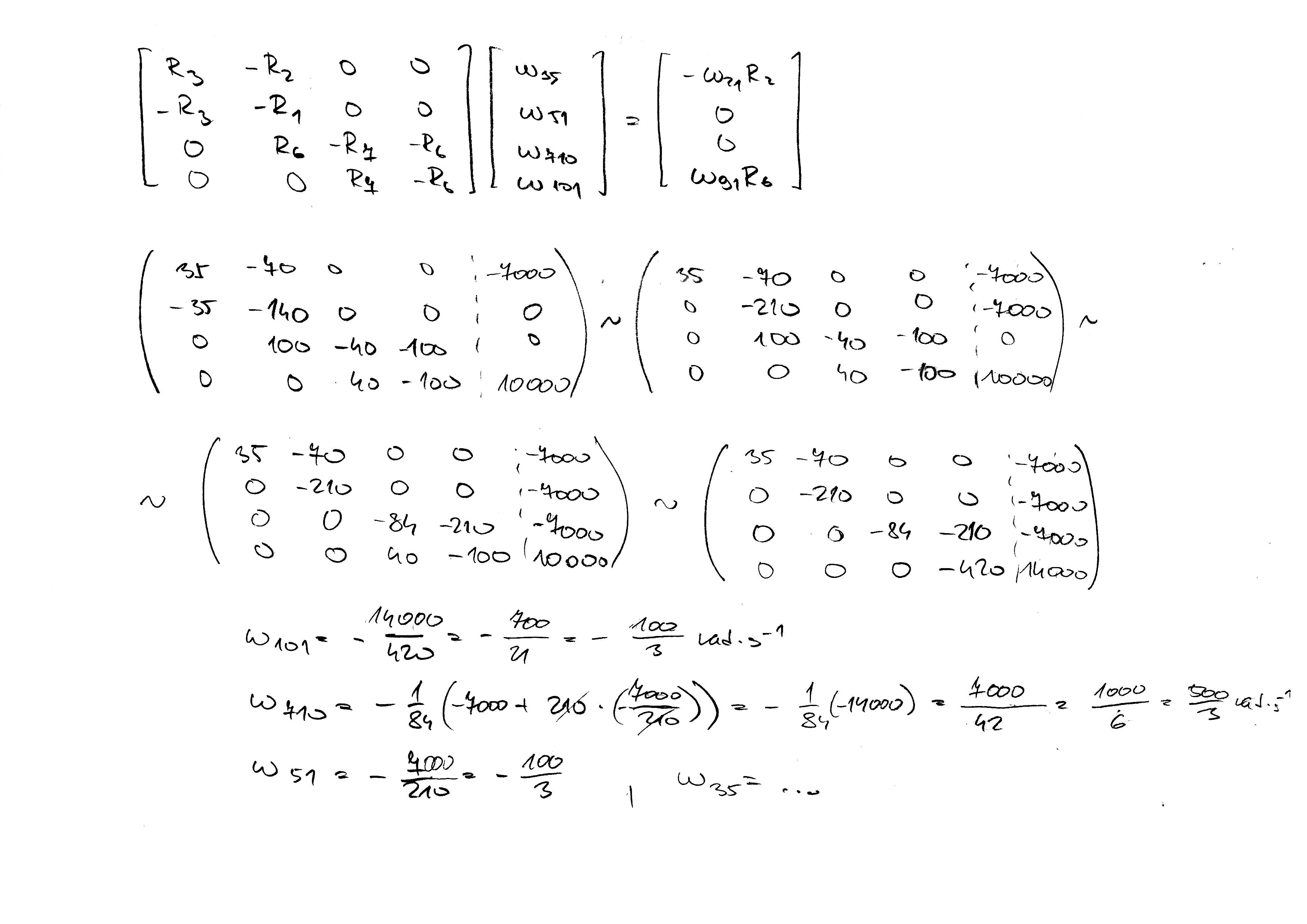
  • Cvičení 6: Obecný rovinný pohyb (ORP)/Složený pohyb.

    • Ručně řešený příklad Př.1 lze stáhnout zde, zde a zde.

    • Ručně řešený příklad Př.2 lze stáhnout zde, zde a zde.

    • Ručně řešený příklad Př.3 lze stáhnout zde a zde.

    • Ručně řešený příklad Př.4 lze stáhnout zde.

    • Ručně řešený příklad Př.5 lze stáhnout zde.

  • Cvičení 7: Složený pohyb.

    • Ručně řešený příklad Př.1 lze stáhnout zde, zde, zde a zde.

    • Ručně řešený příklad Př.2 lze stáhnout zde, zde, zde, zde a zde.

    • Ručně řešený příklad Př.3 lze stáhnout zde, zde, zde a zde.

  • Cvičení 8: Složený pohyb.

  • Cvičení 9: Mechanismy s vačkami.

    • Ručně řešený příklad Př.1 lze stáhnout zde, zde, zde, zde a zde.

    • Ručně řešený příklad Př.2 lze stáhnout zde, zde a zde.

    • Ručně řešený příklad Př.3 lze stáhnout zde a zde.

    • Ručně řešený příklad Př.4 lze stáhnout zde, zde a zde.

    • Ručně řešený příklad Př.5 lze stáhnout zde, zde, zde, zde, zde, zde a zde.

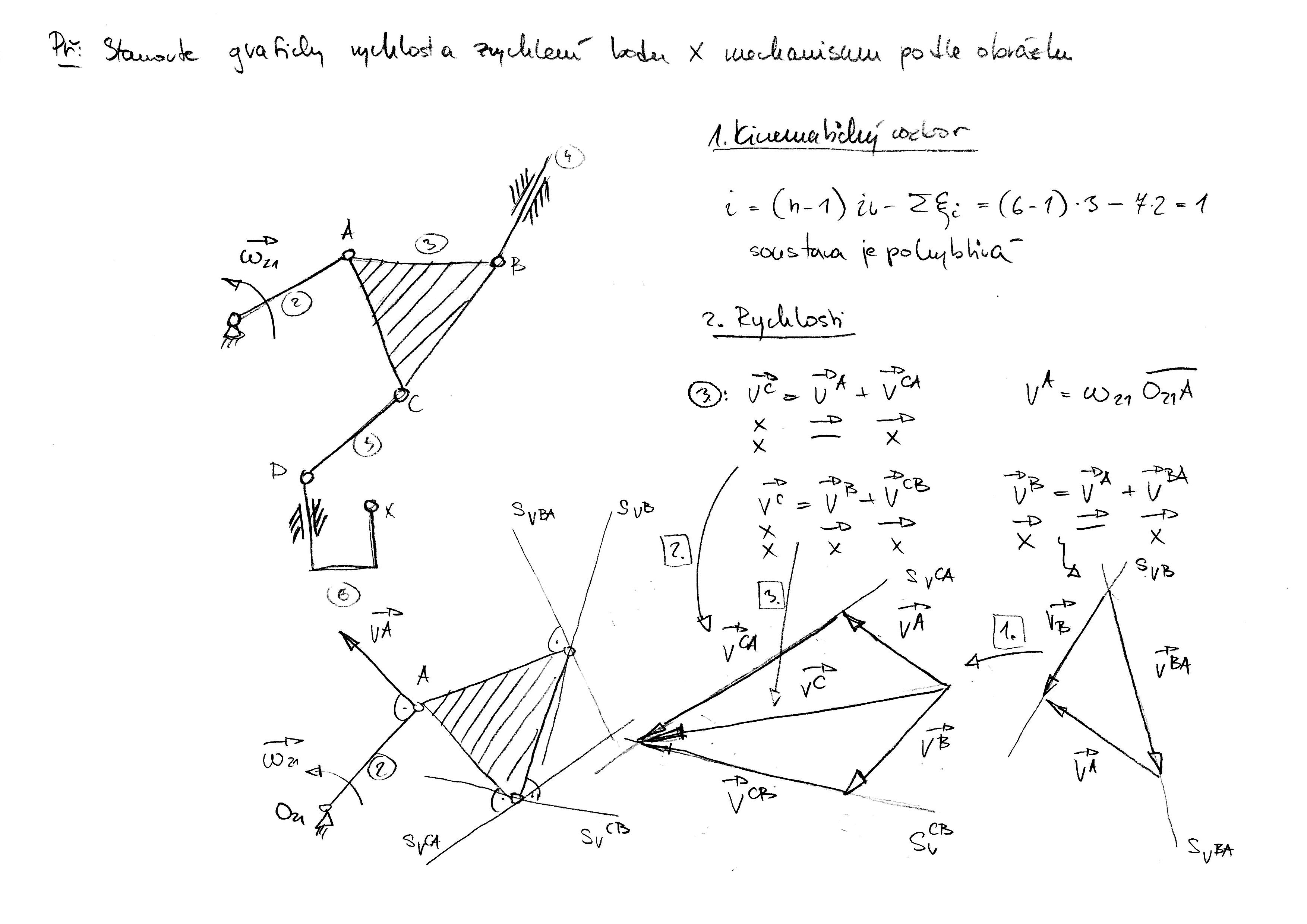
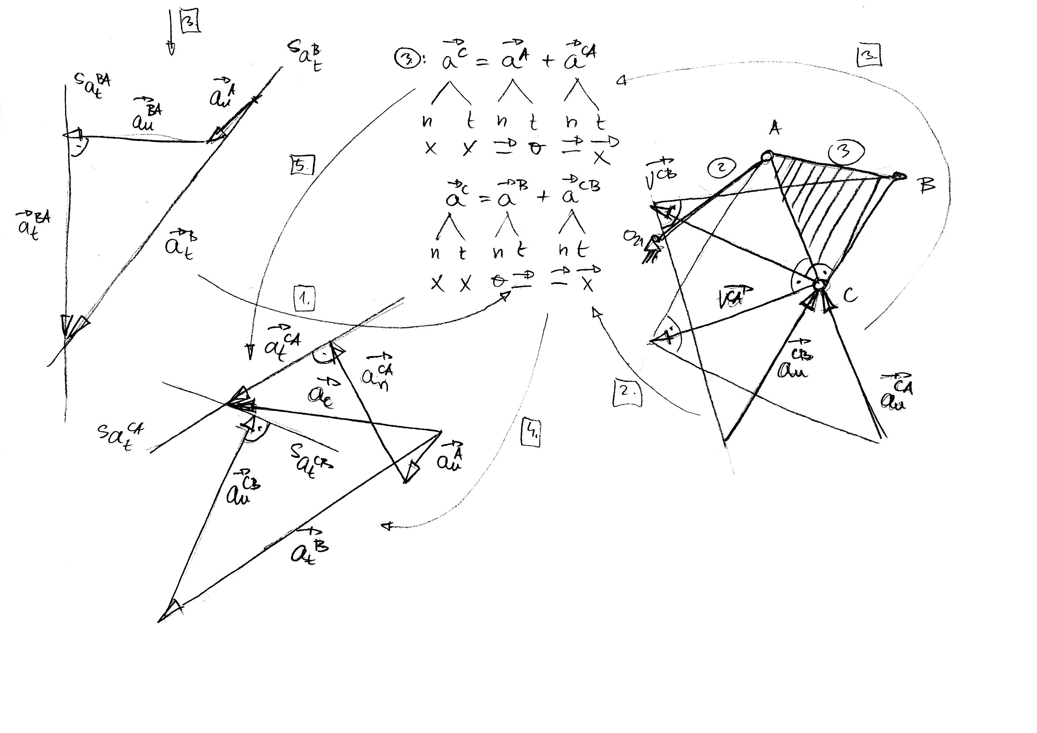
  • Cvičení 10: Mechanismy.

    • Ručně řešený příklad Př.1 lze stáhnout zde a zde.

    • Ručně řešený příklad Př.2 lze stáhnout zde, zde a zde.

    • Ručně řešený příklad Př.3 lze stáhnout zde, zde, zde a zde. Ukázka numerického řešení v jazyce Python zde a grafy numerického řešení zde, zde.

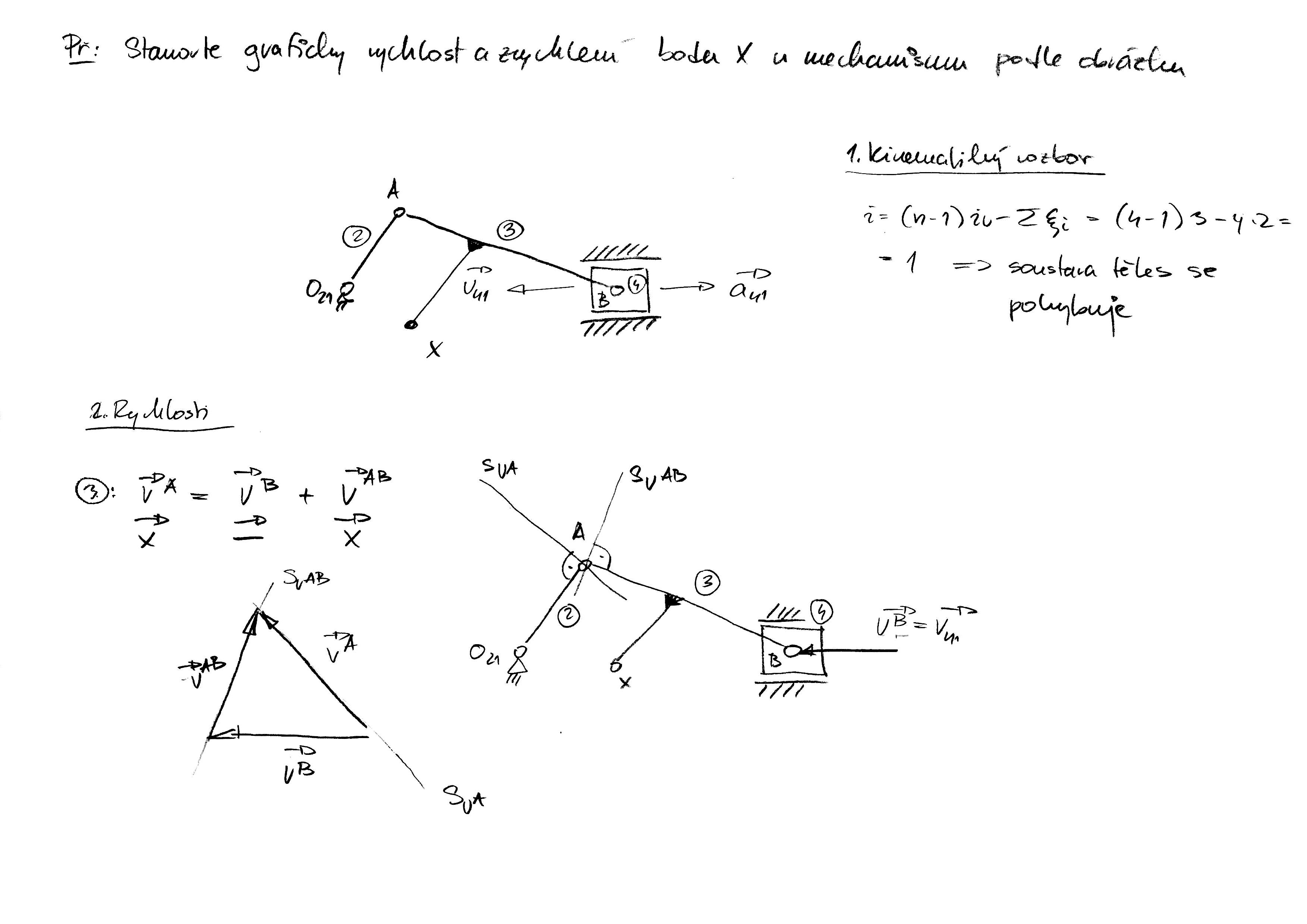
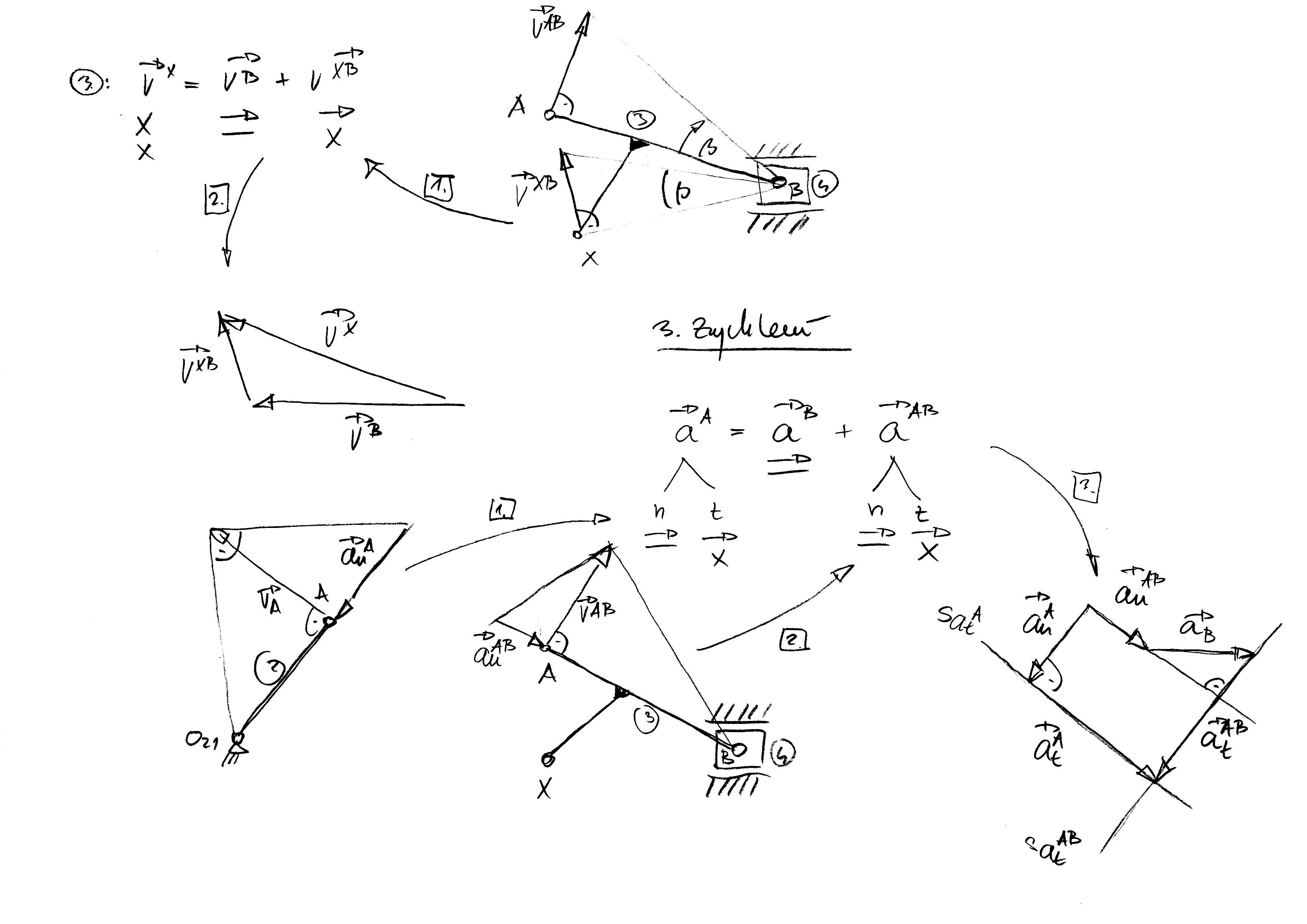
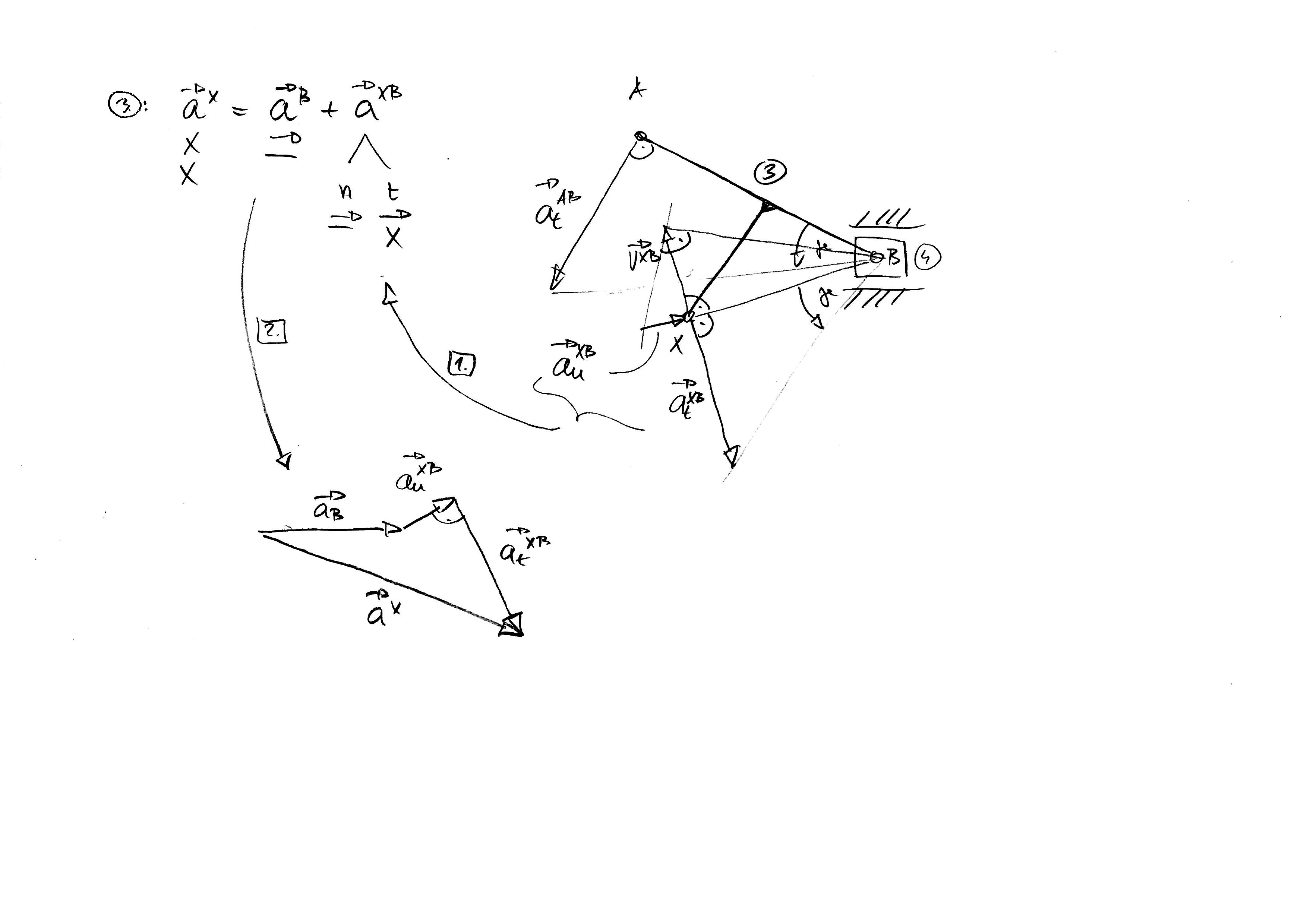
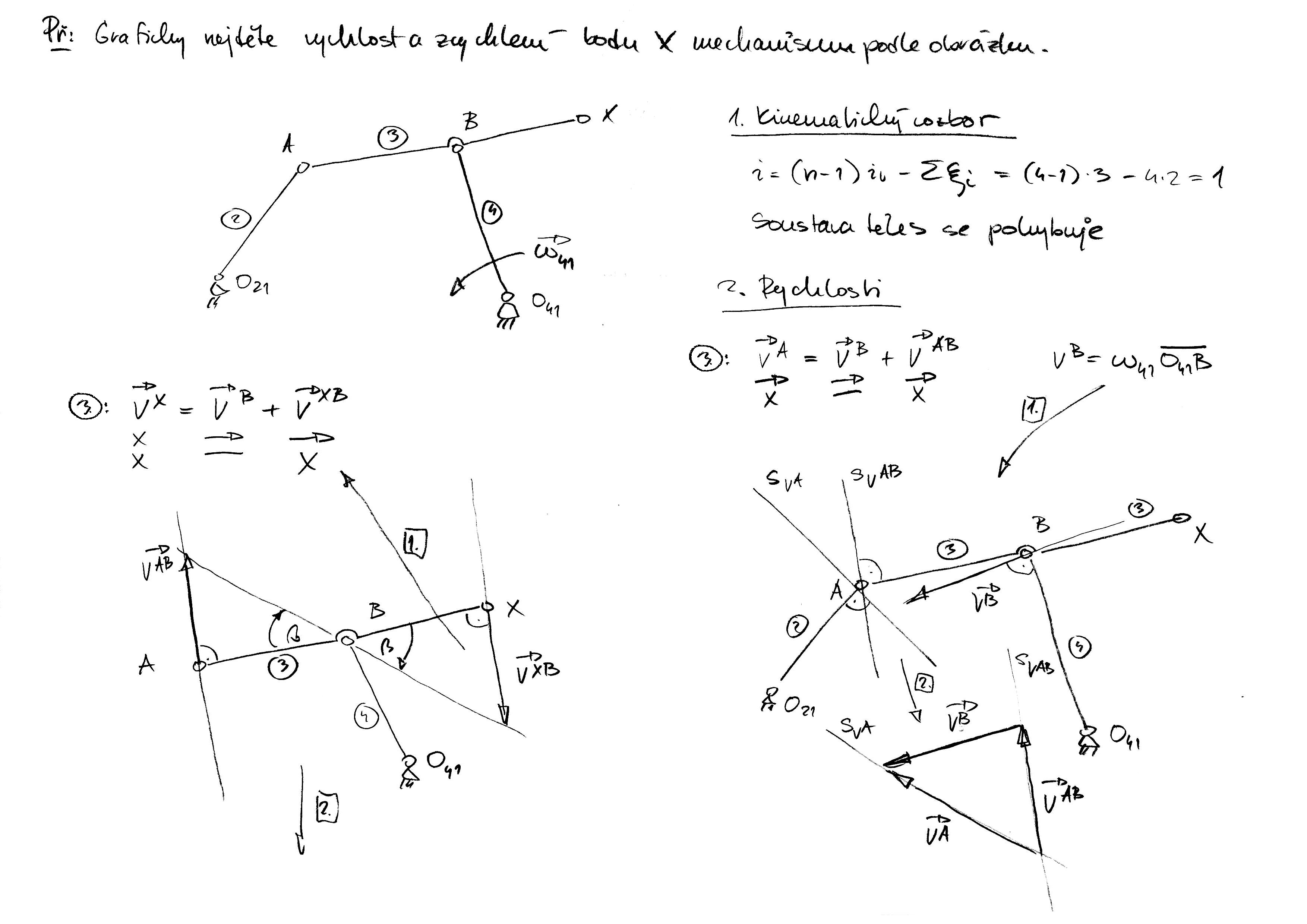
  • Cvičení 11: Mechanismy.

  • Cvičení 12: Současné rotace, planetové mechanismy.
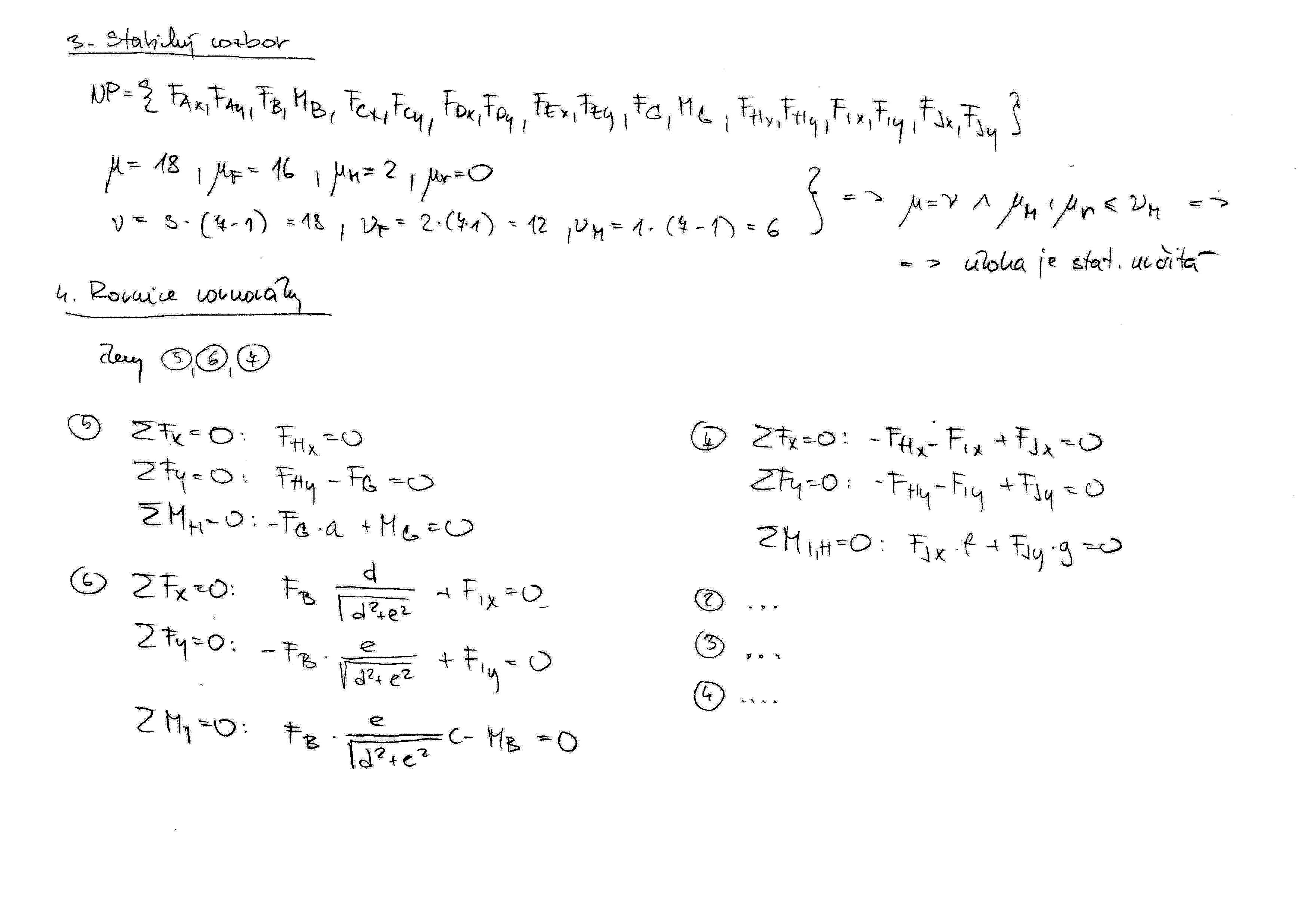
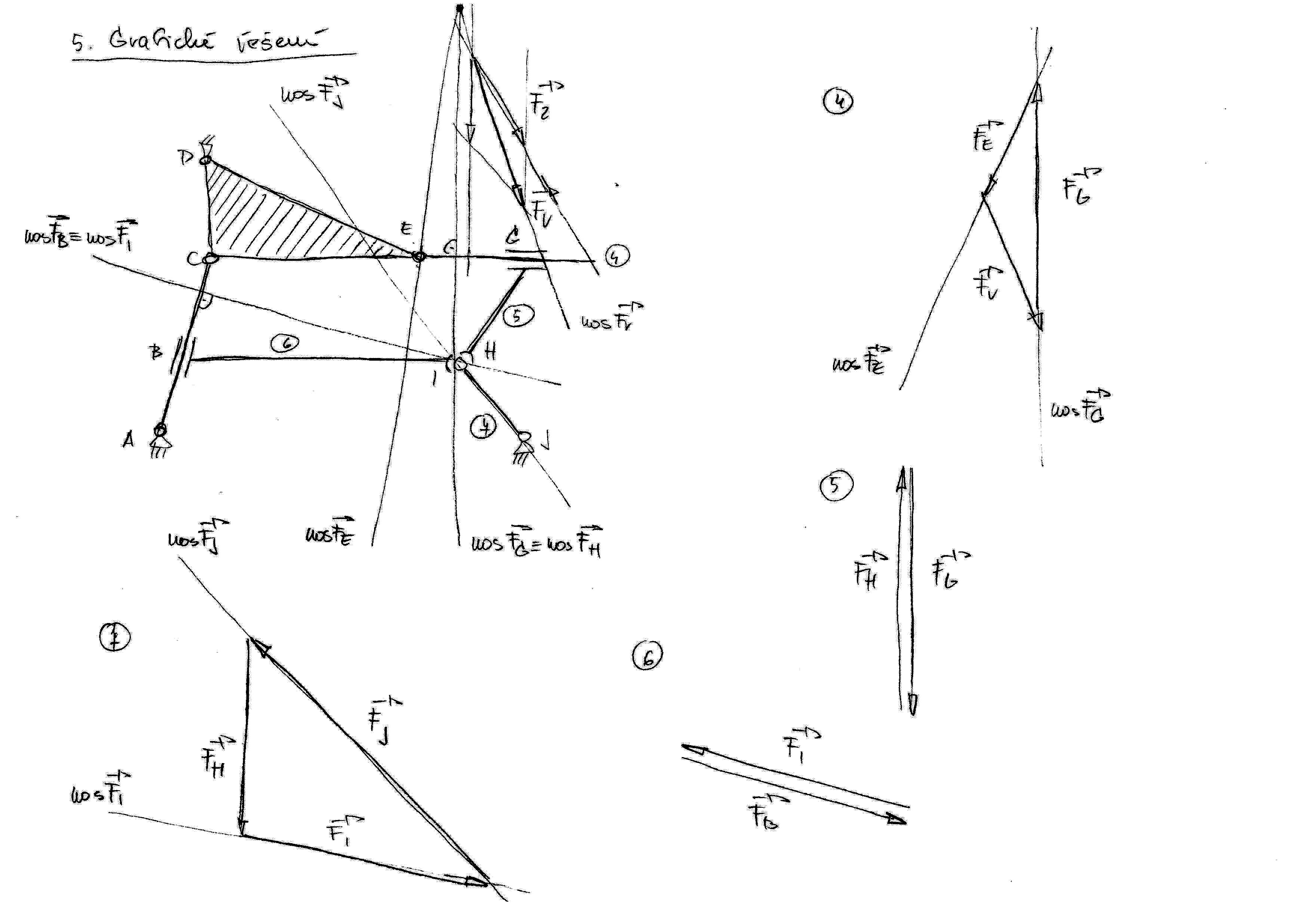
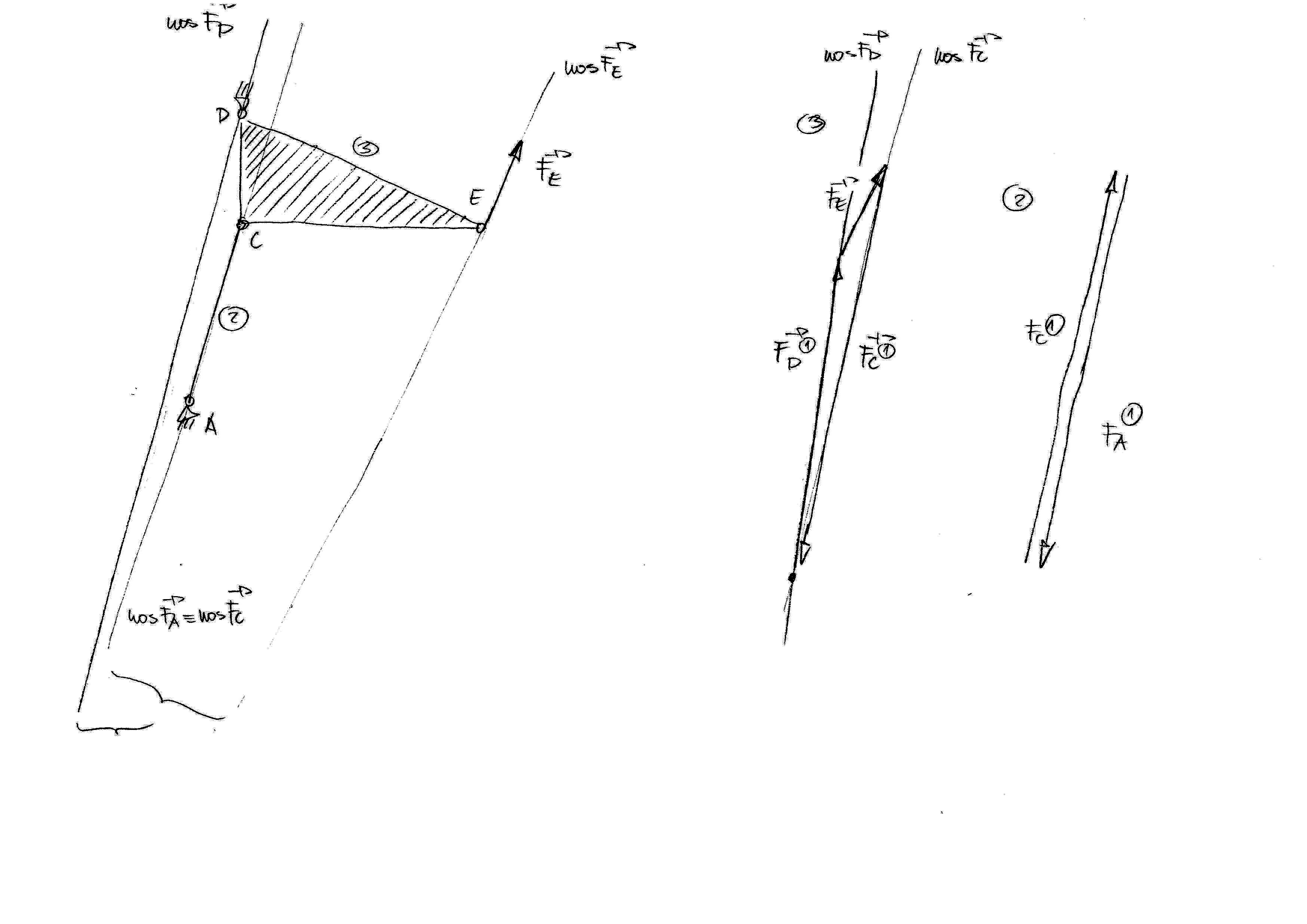
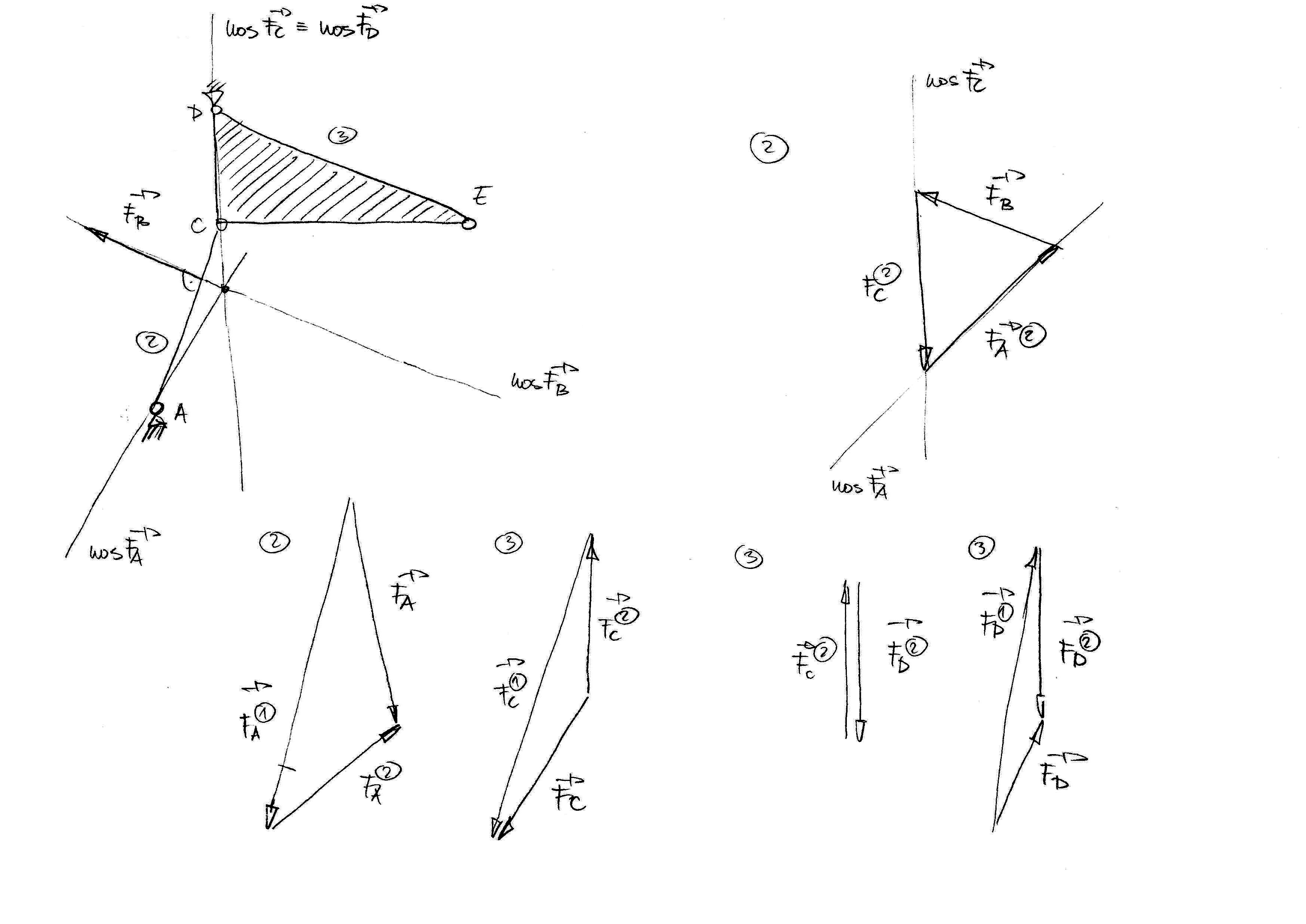
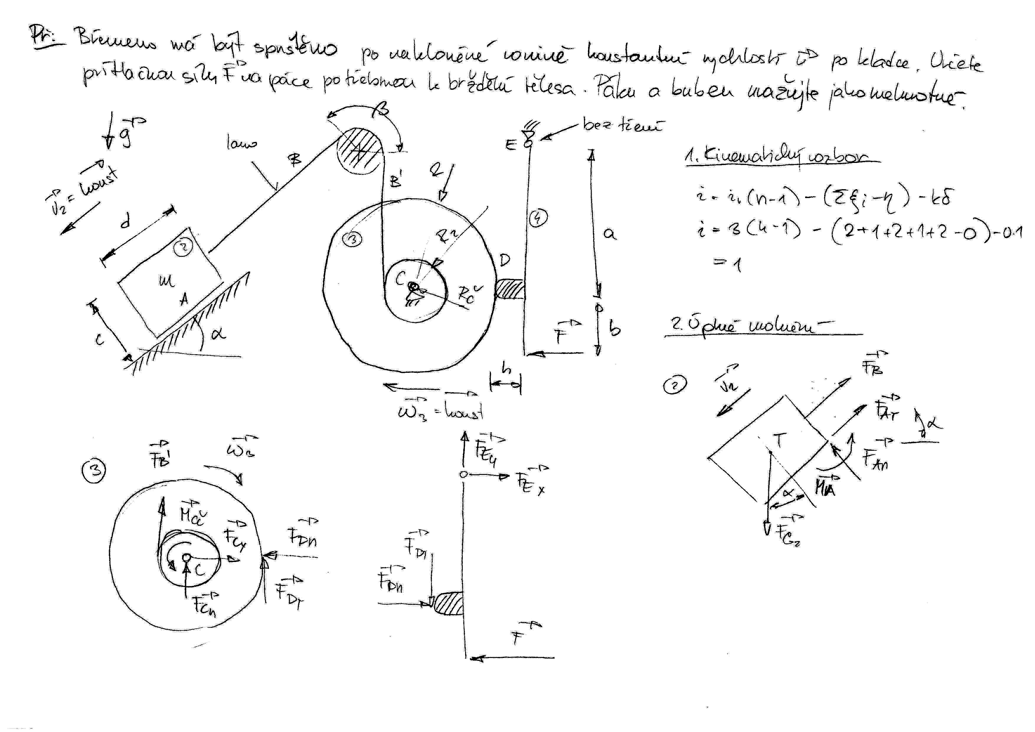
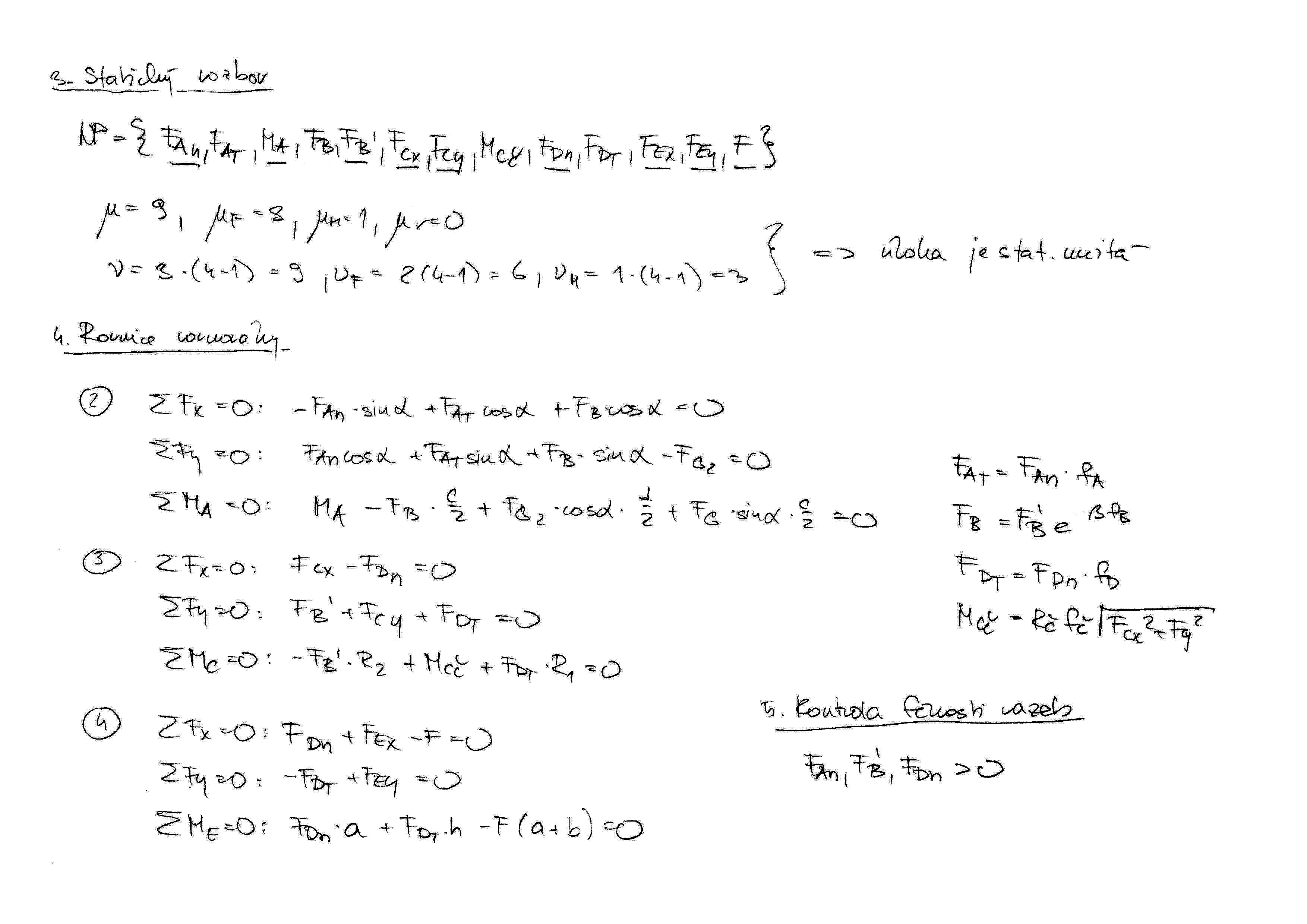
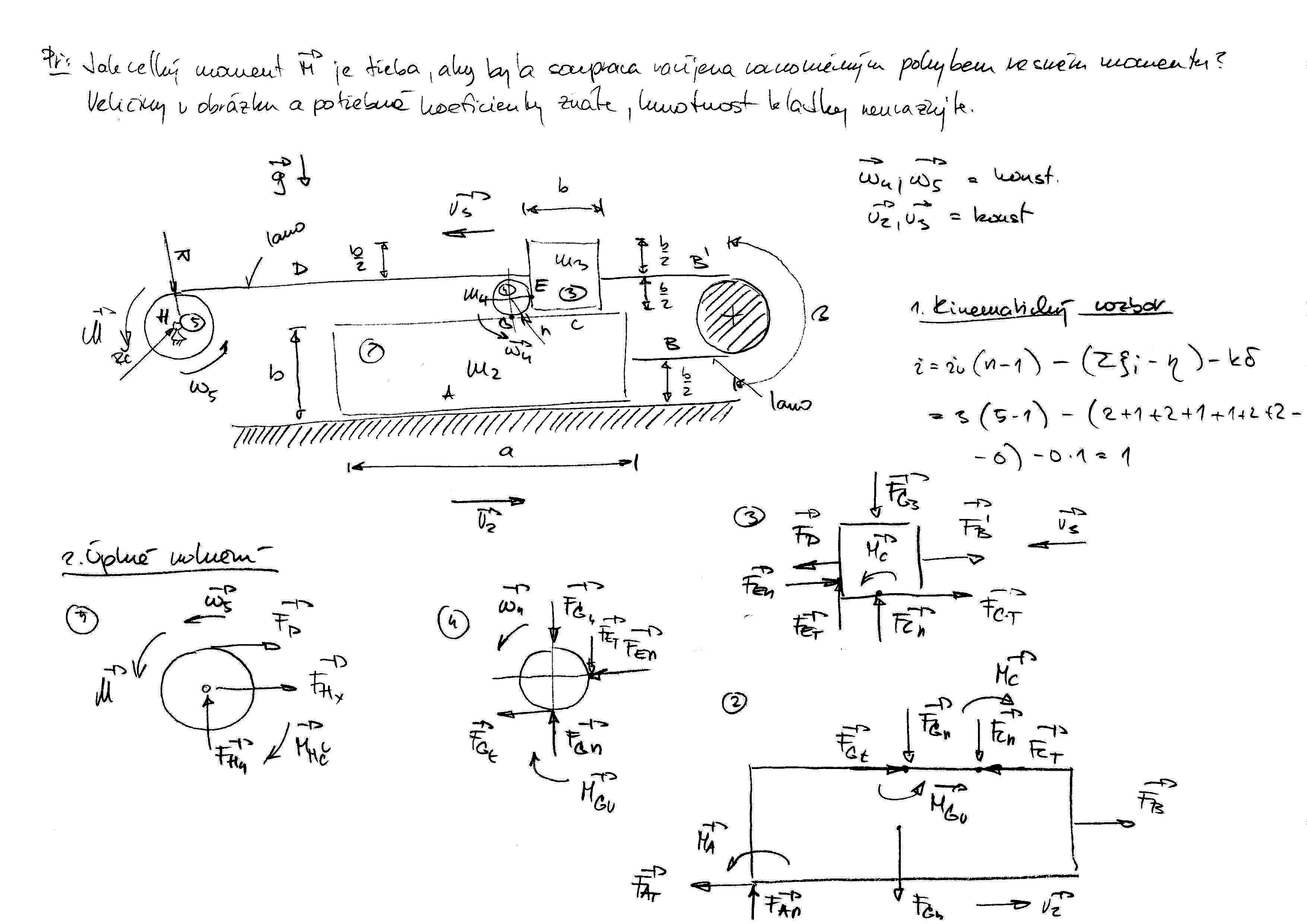
    • Ručně řešený příklad Př.1 lze stáhnout zde a zde.

    • Ručně řešený příklad Př.2 lze stáhnout zde, zde a zde.

Statika

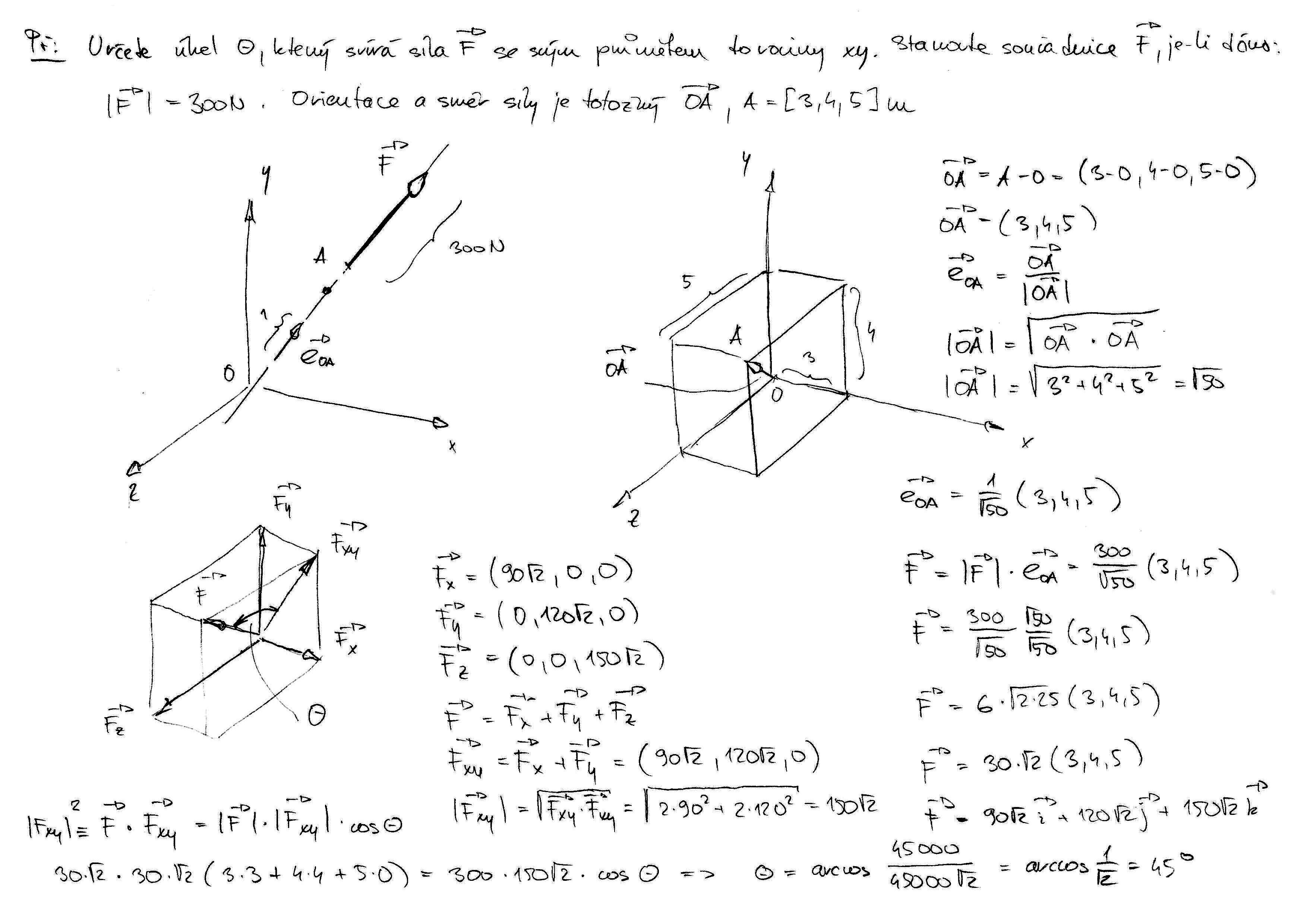
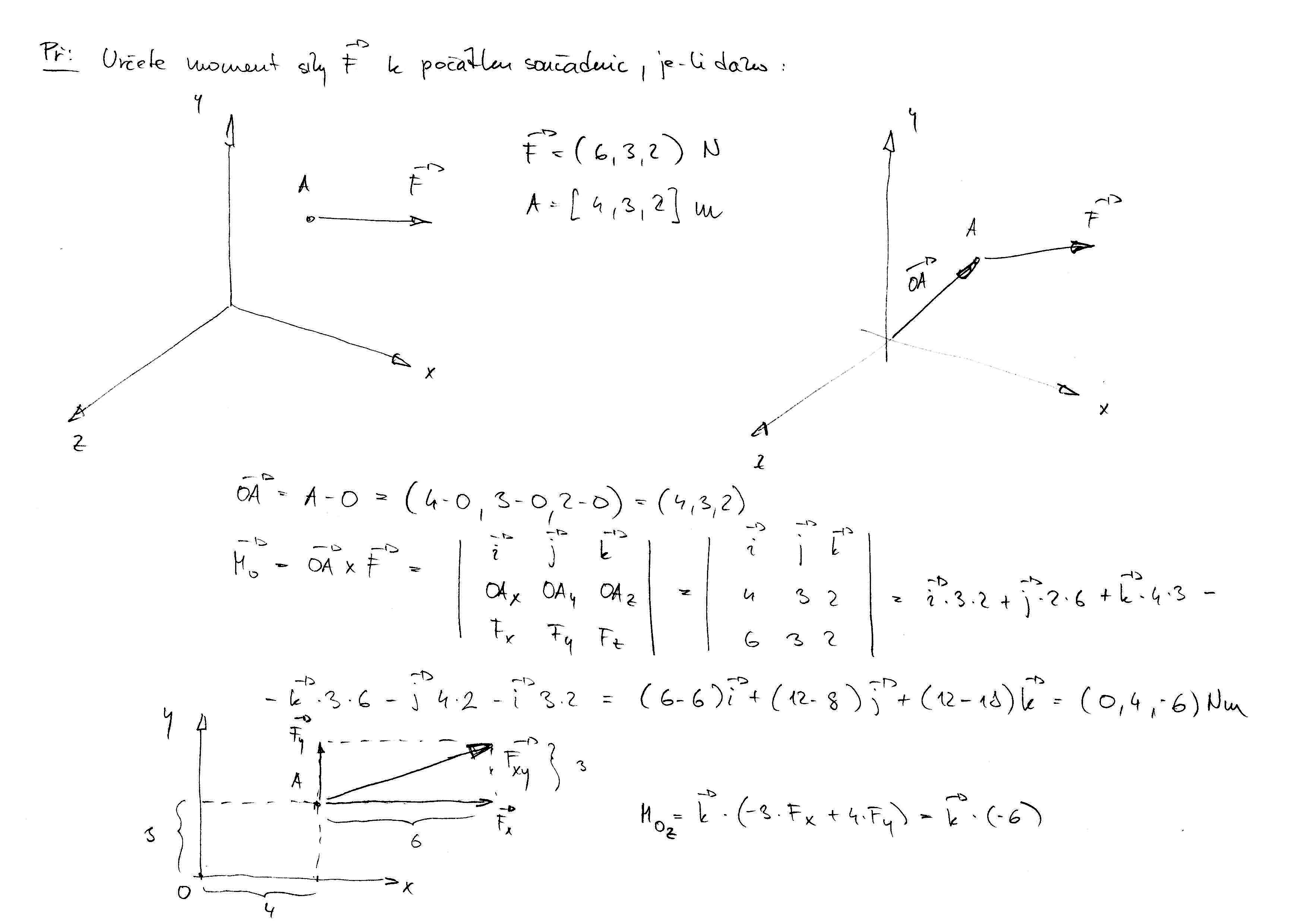
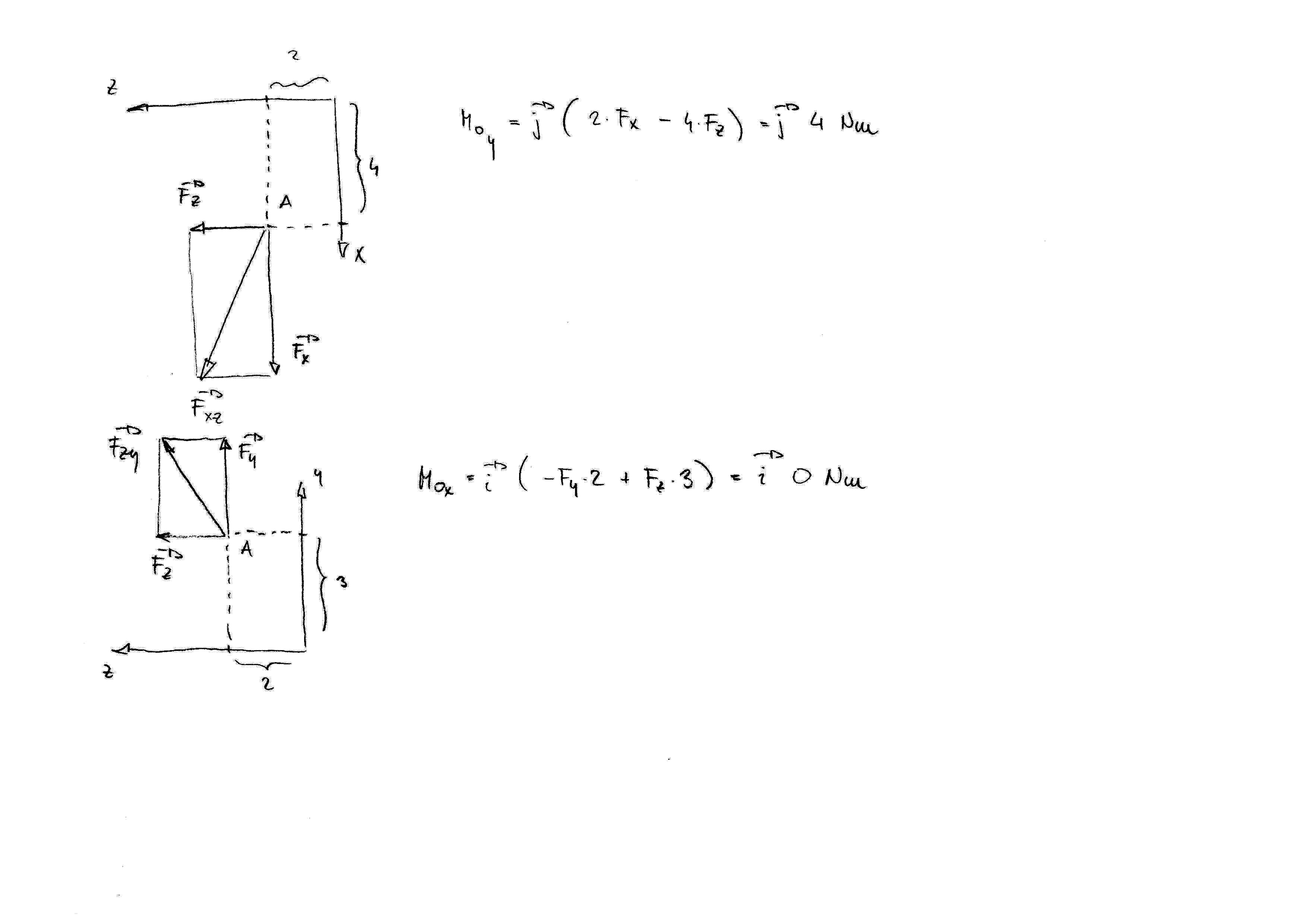
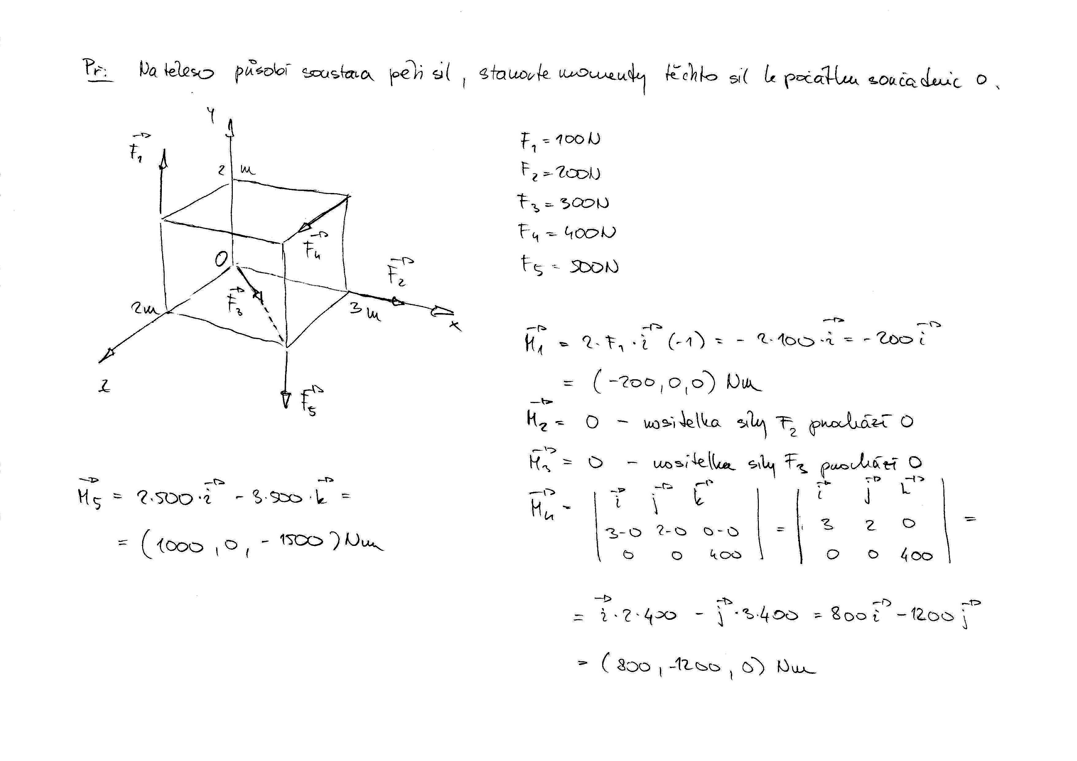
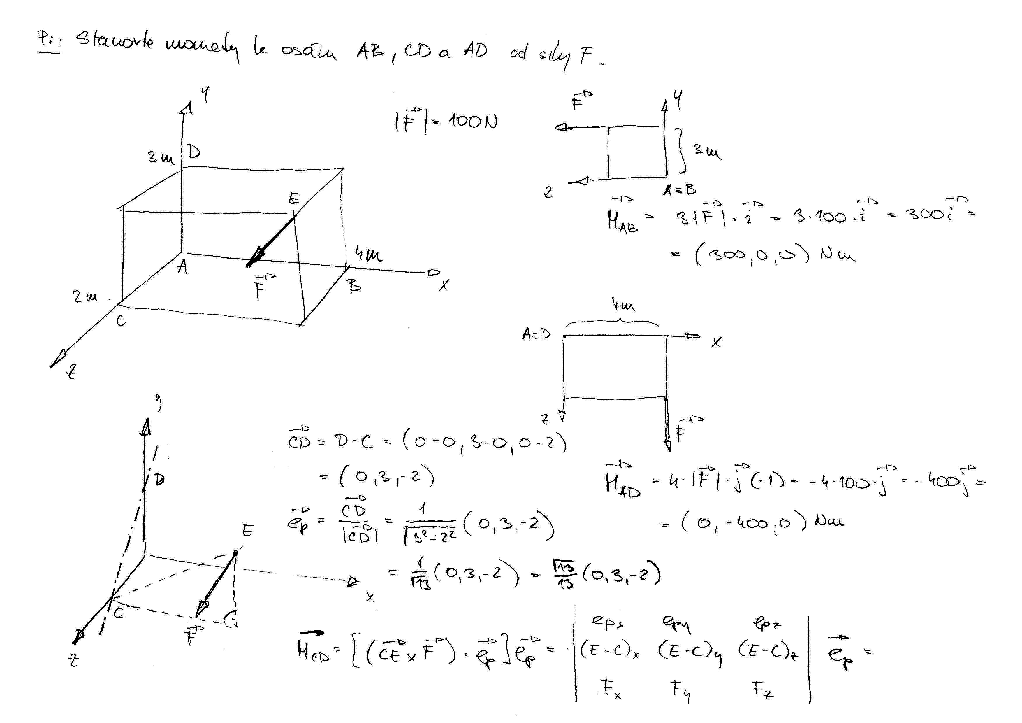
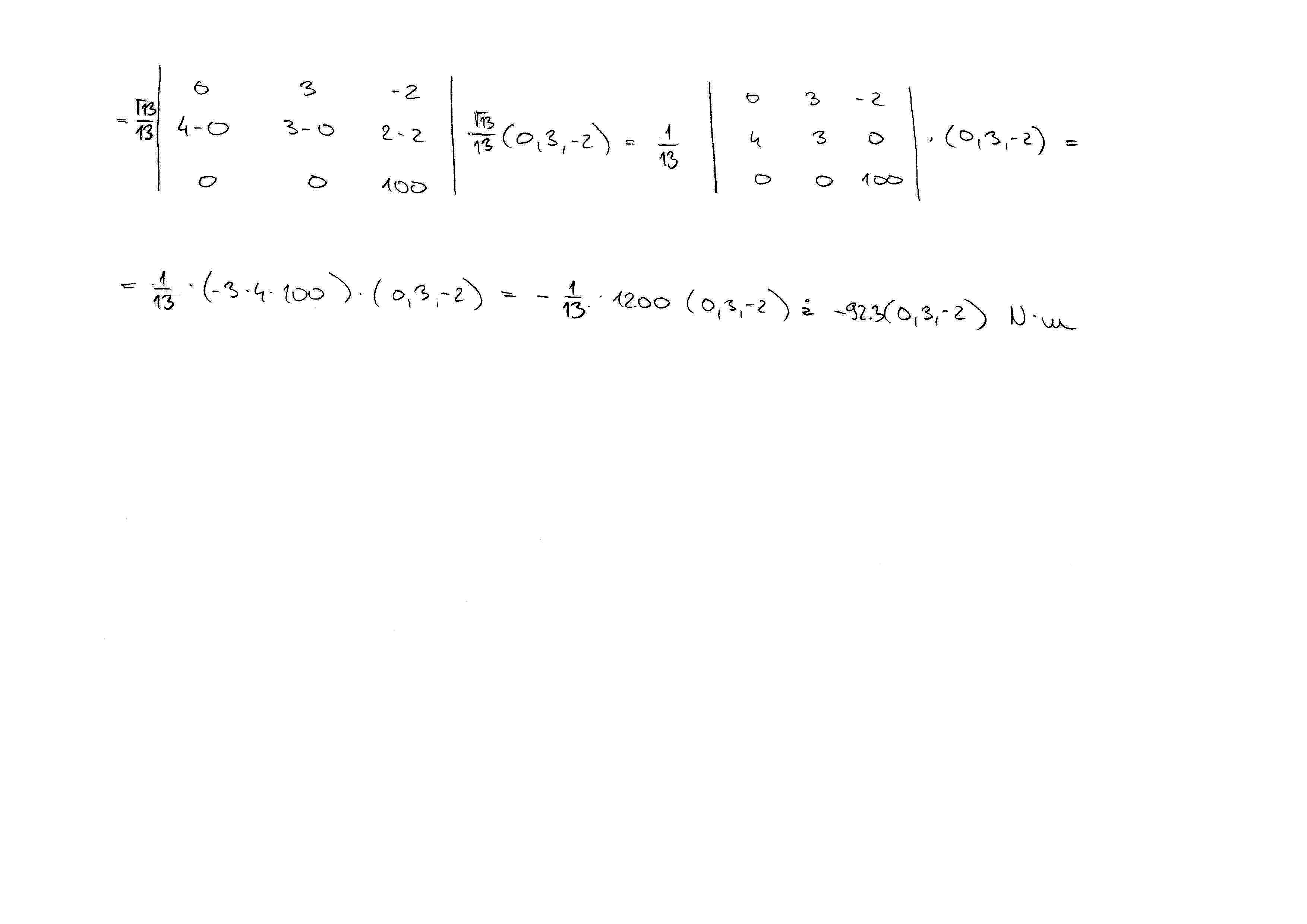
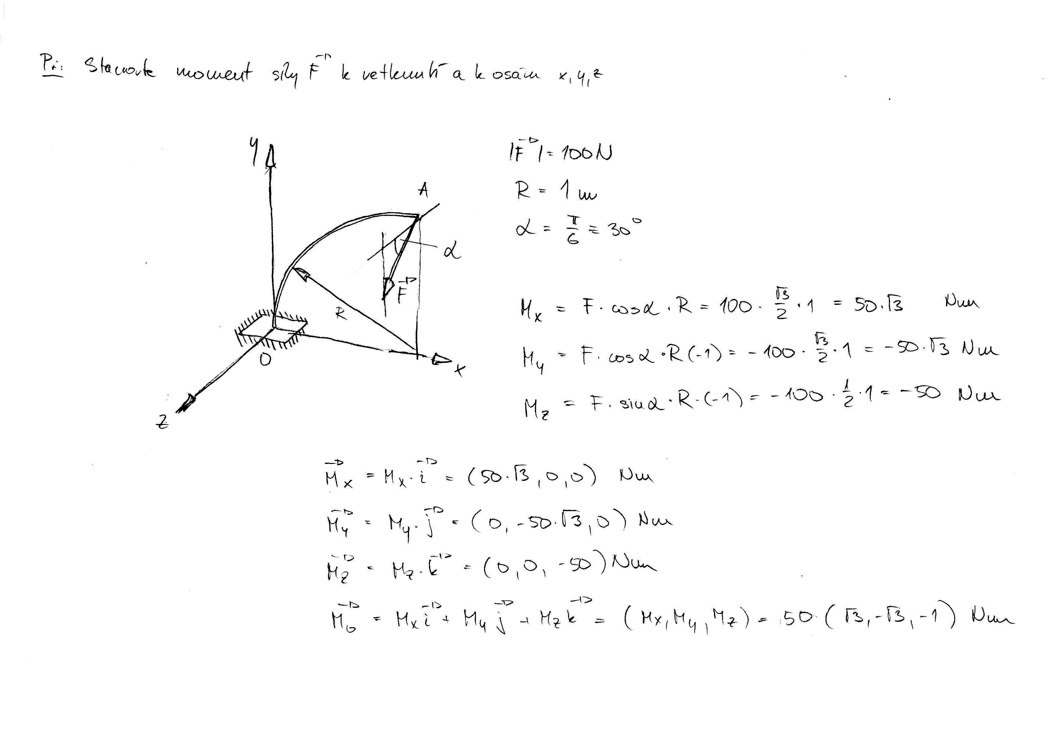
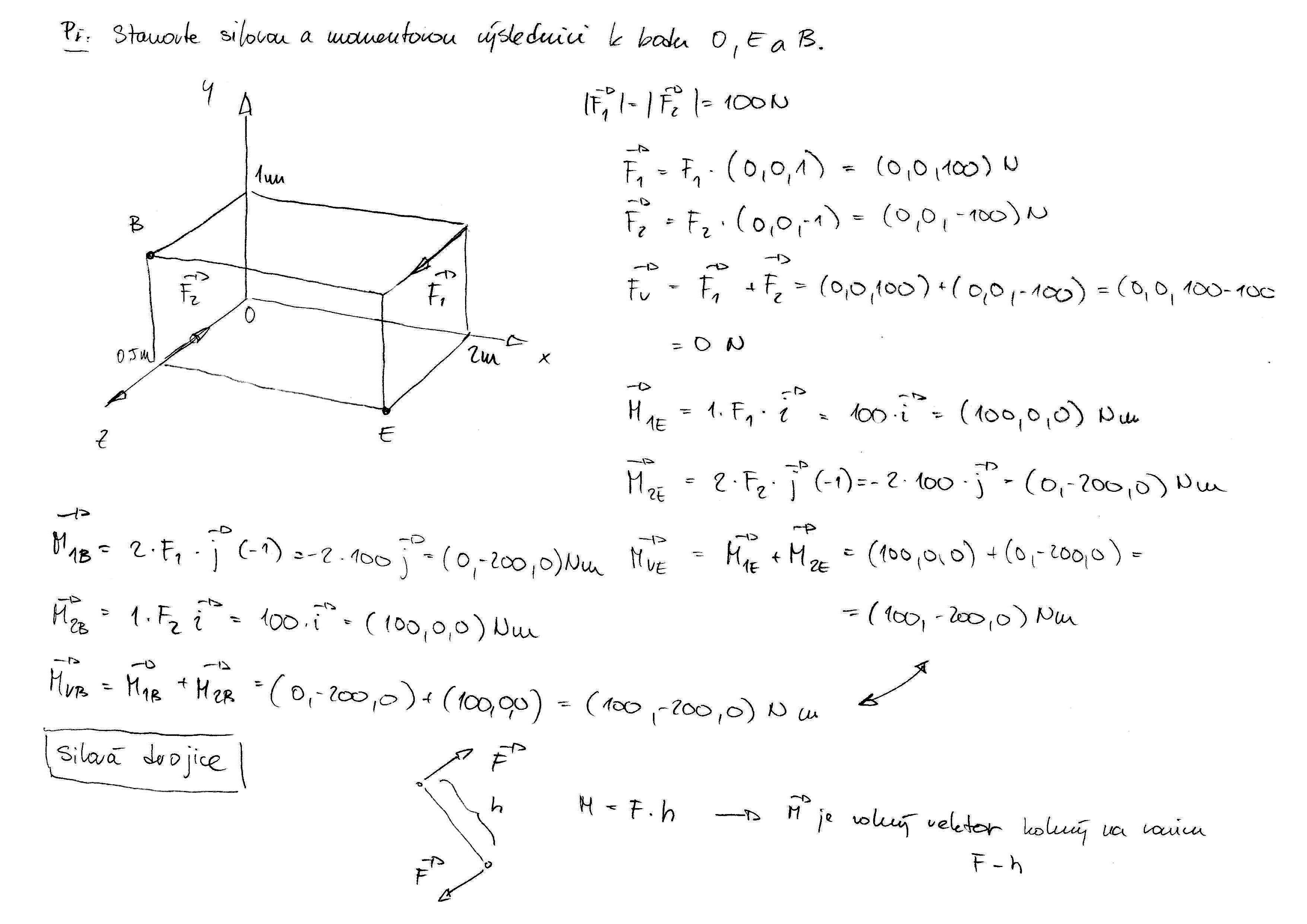
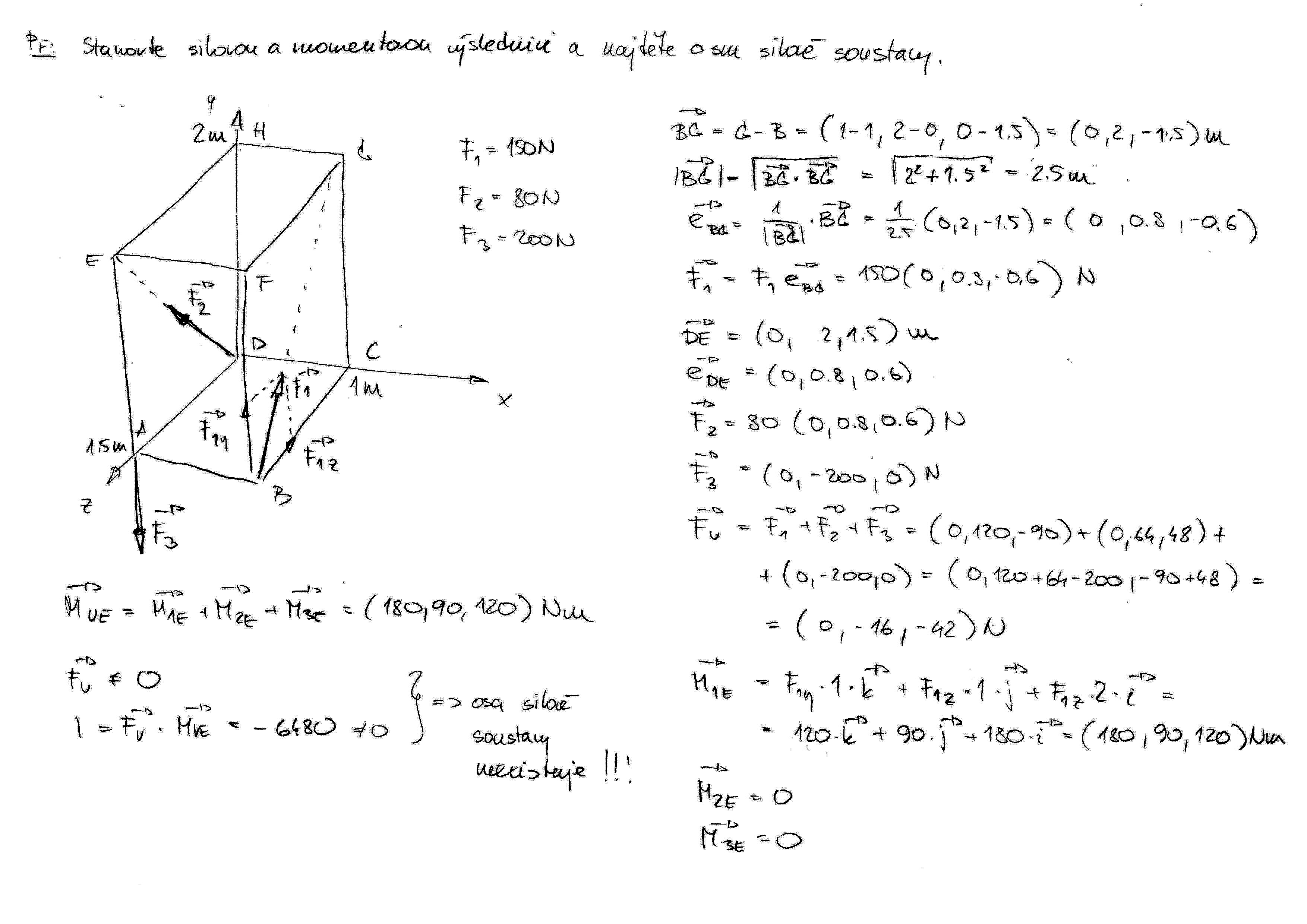
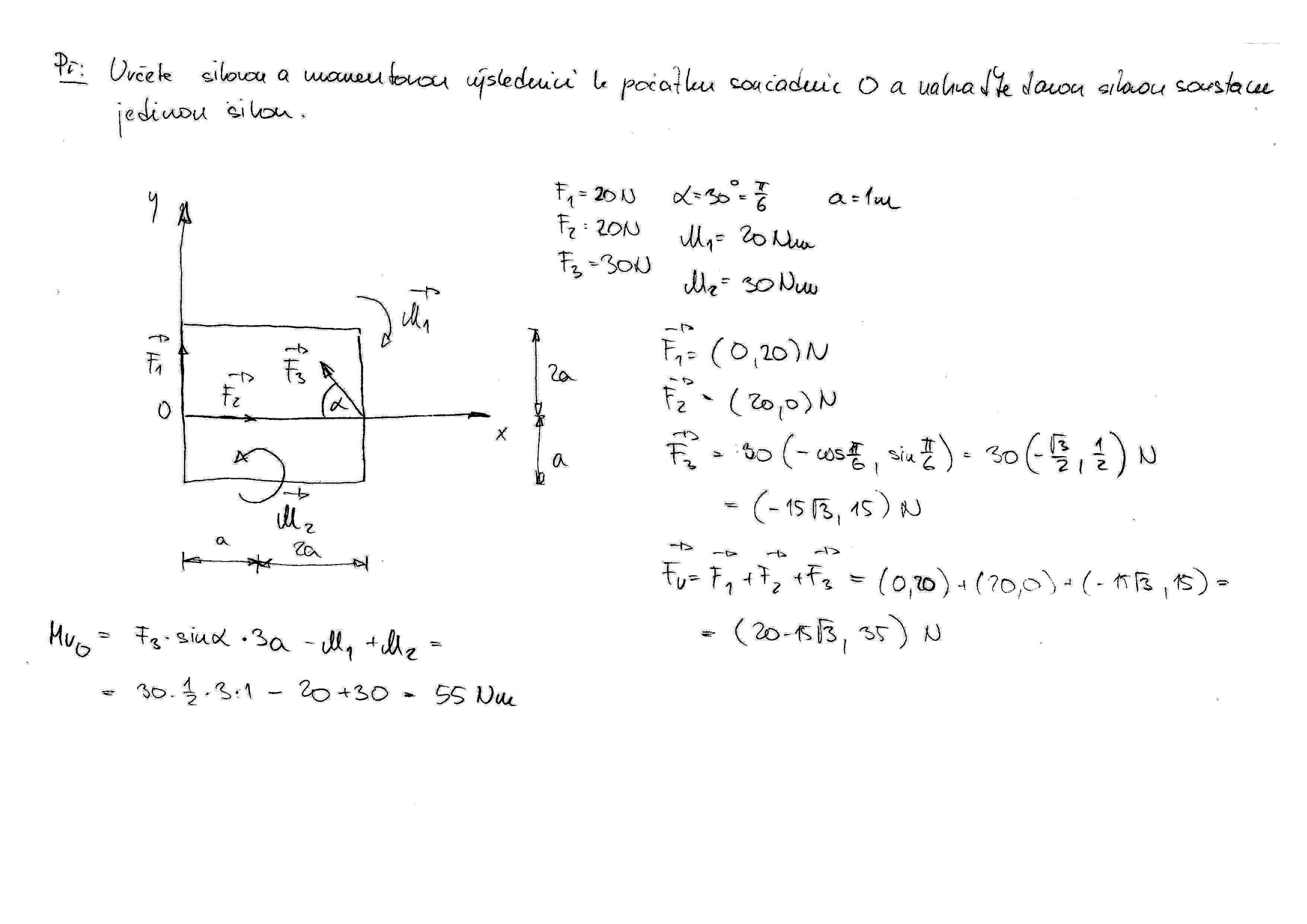
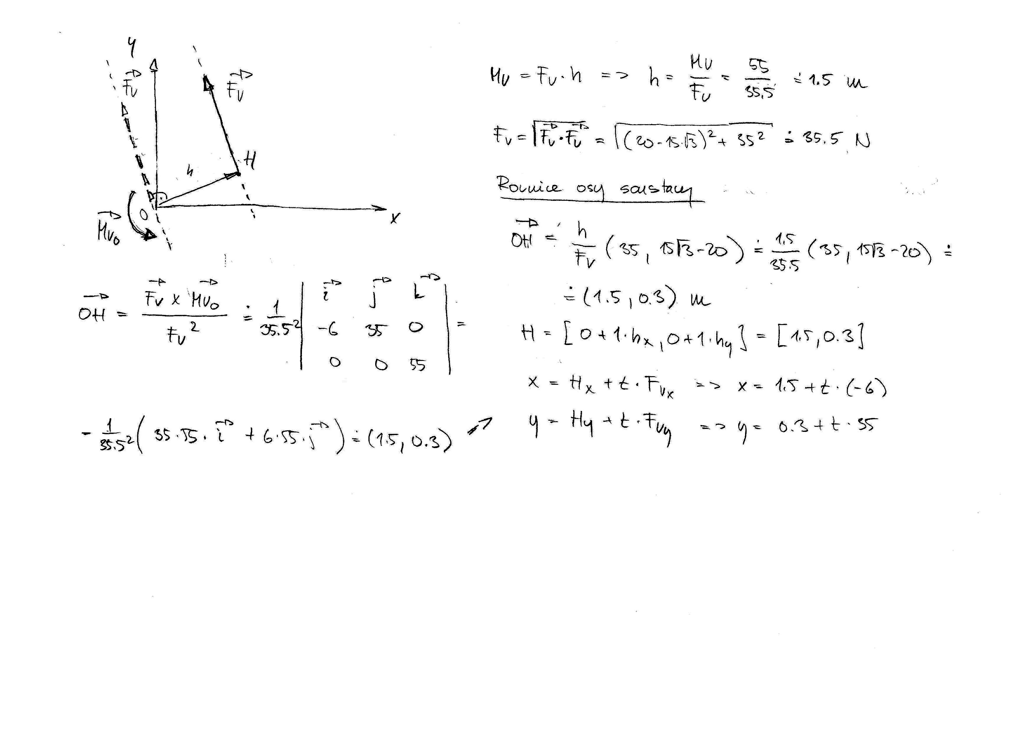
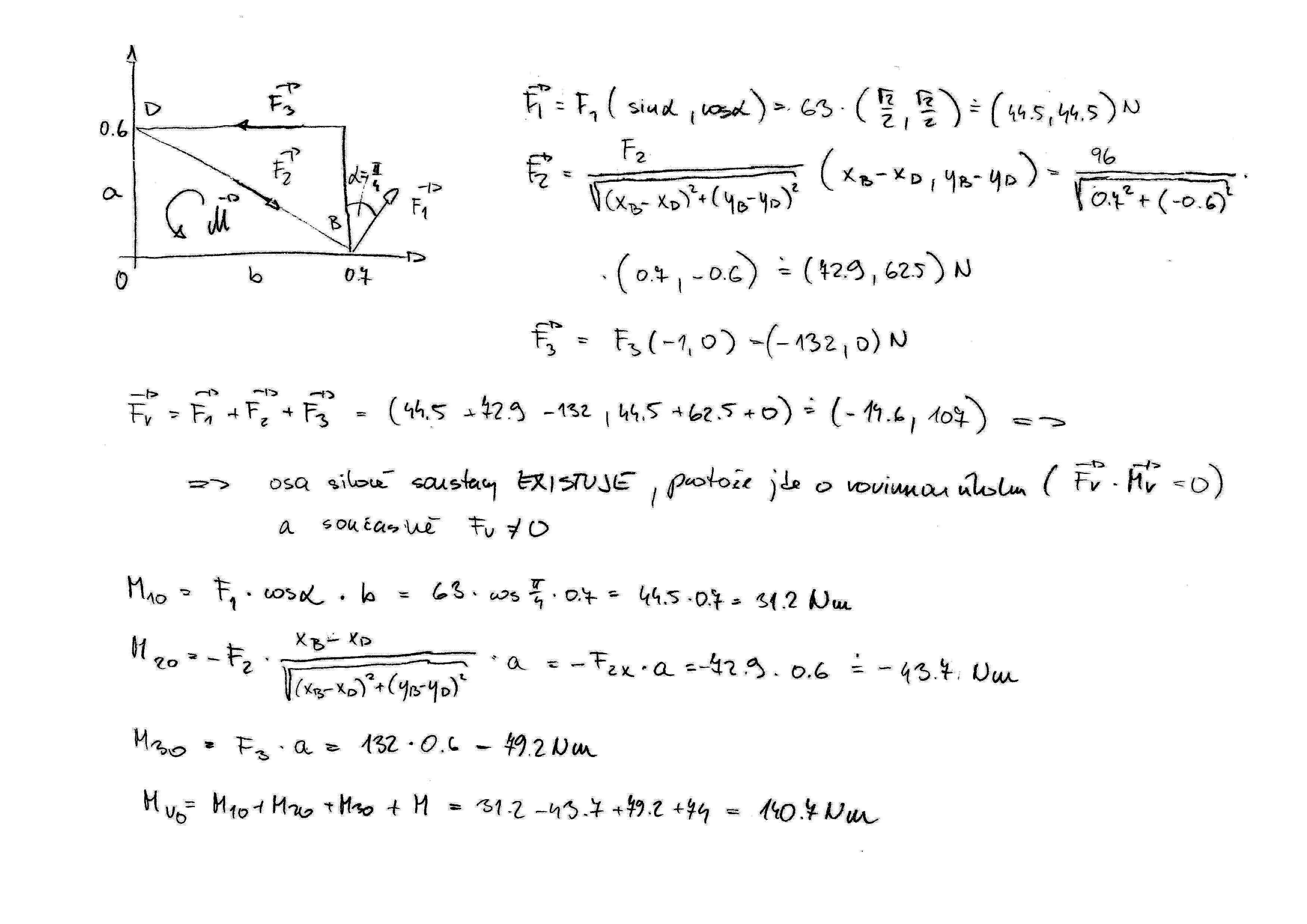
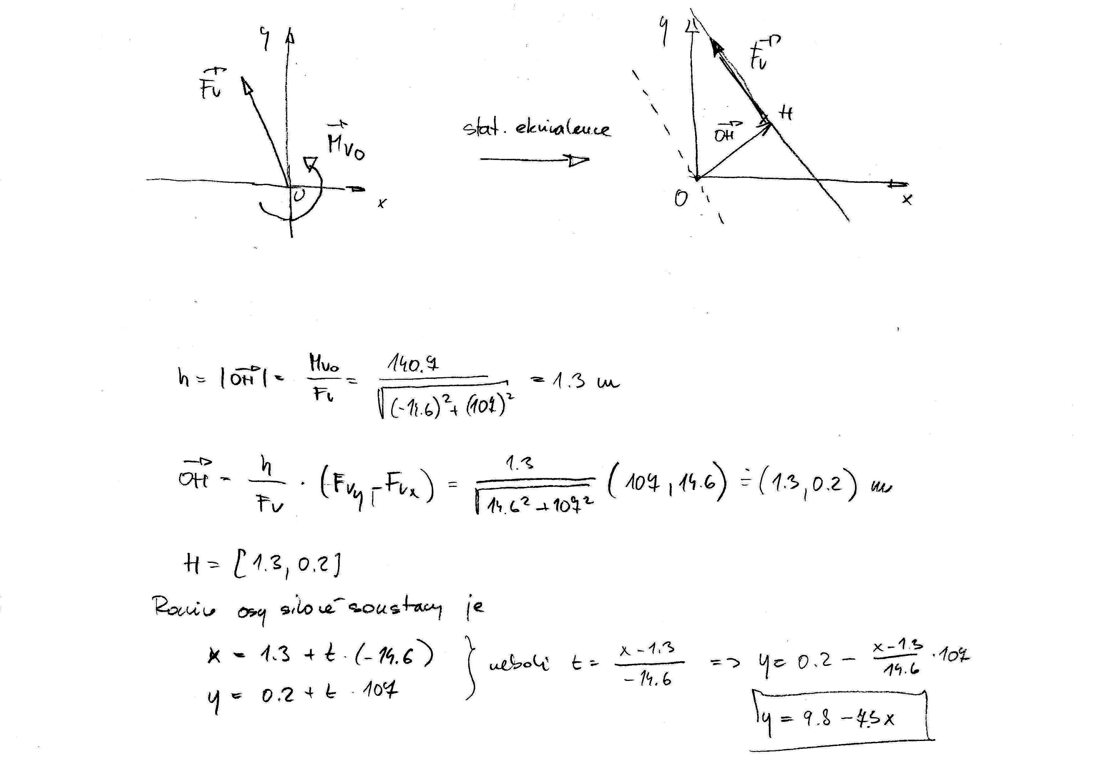
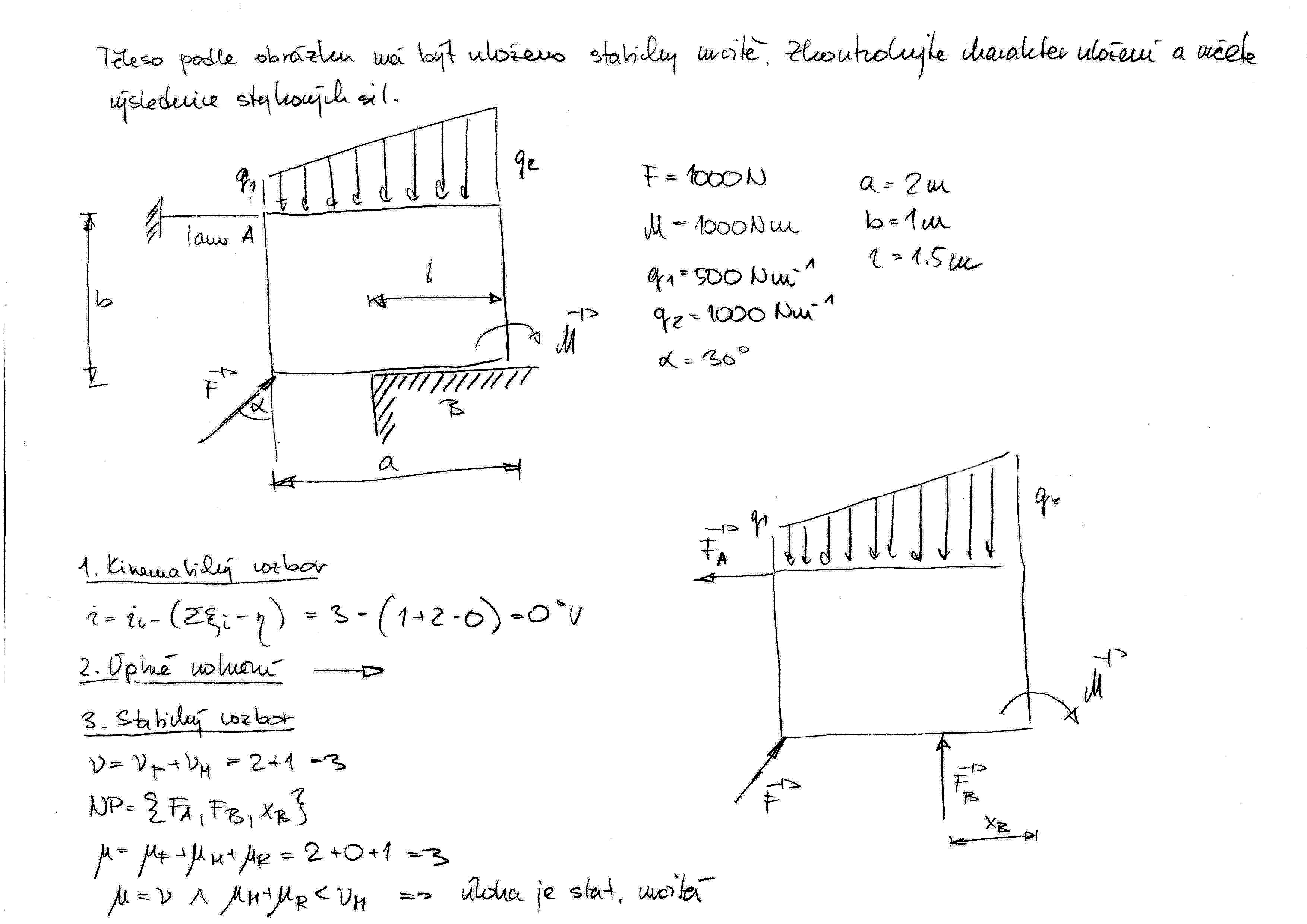
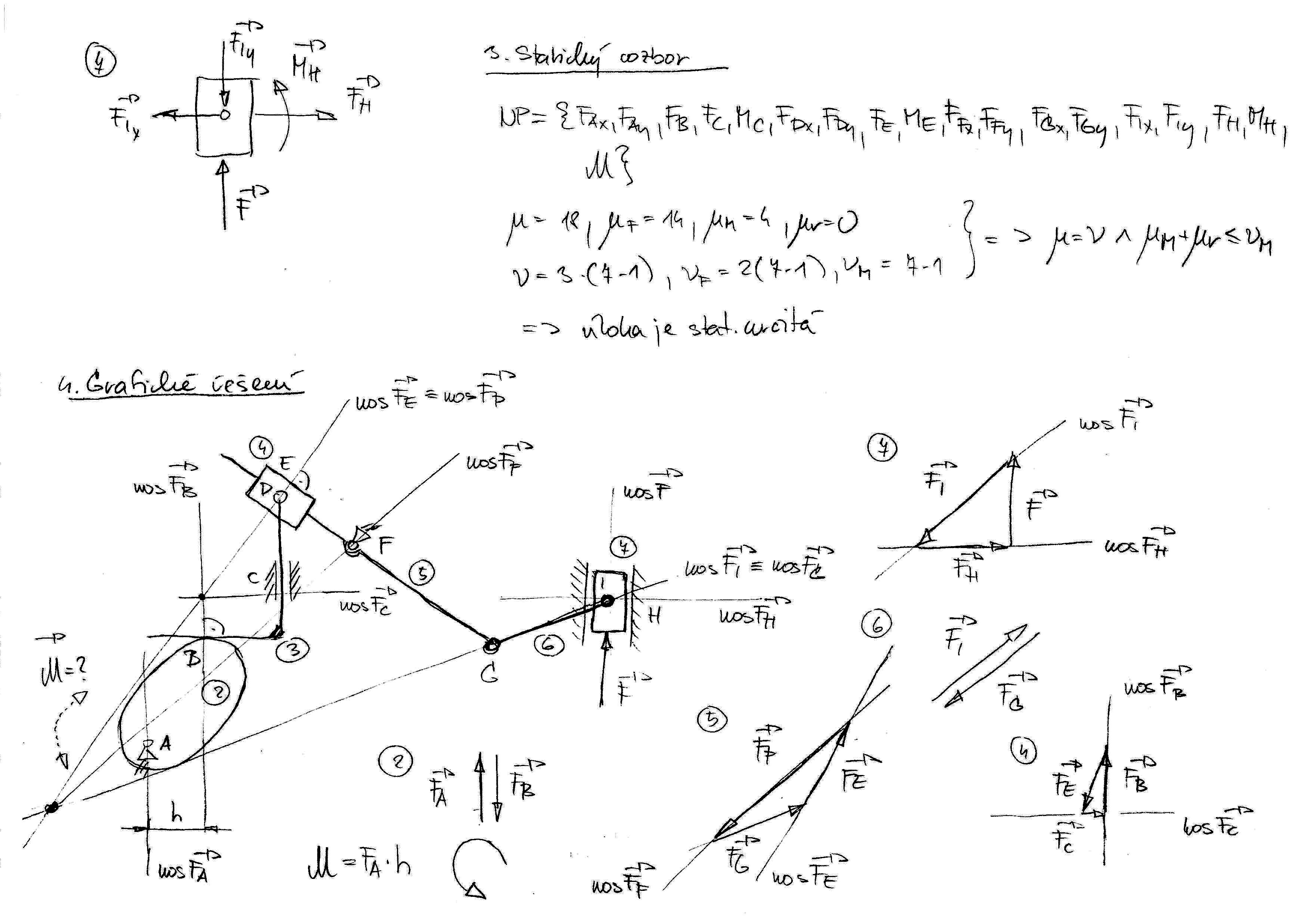
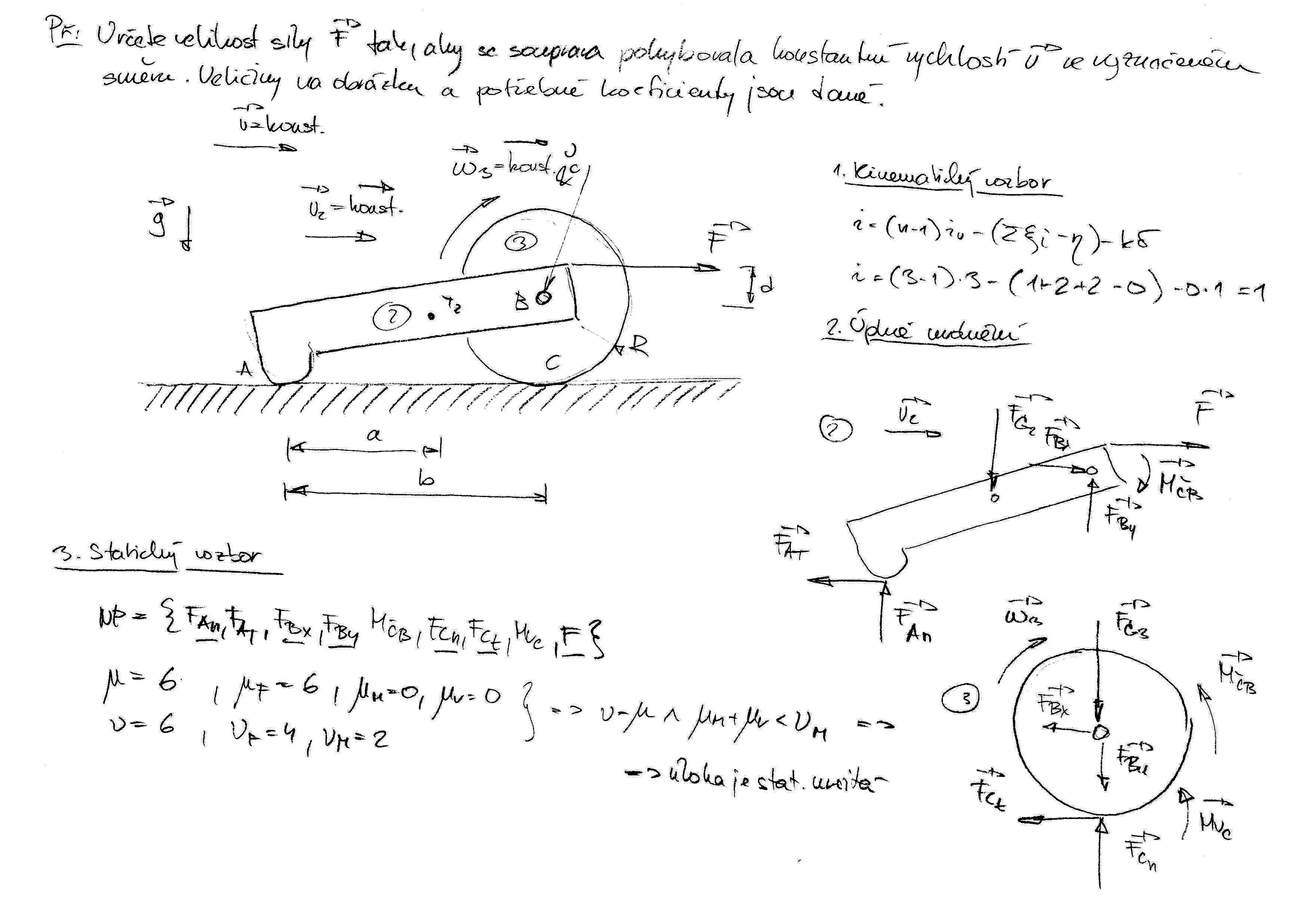
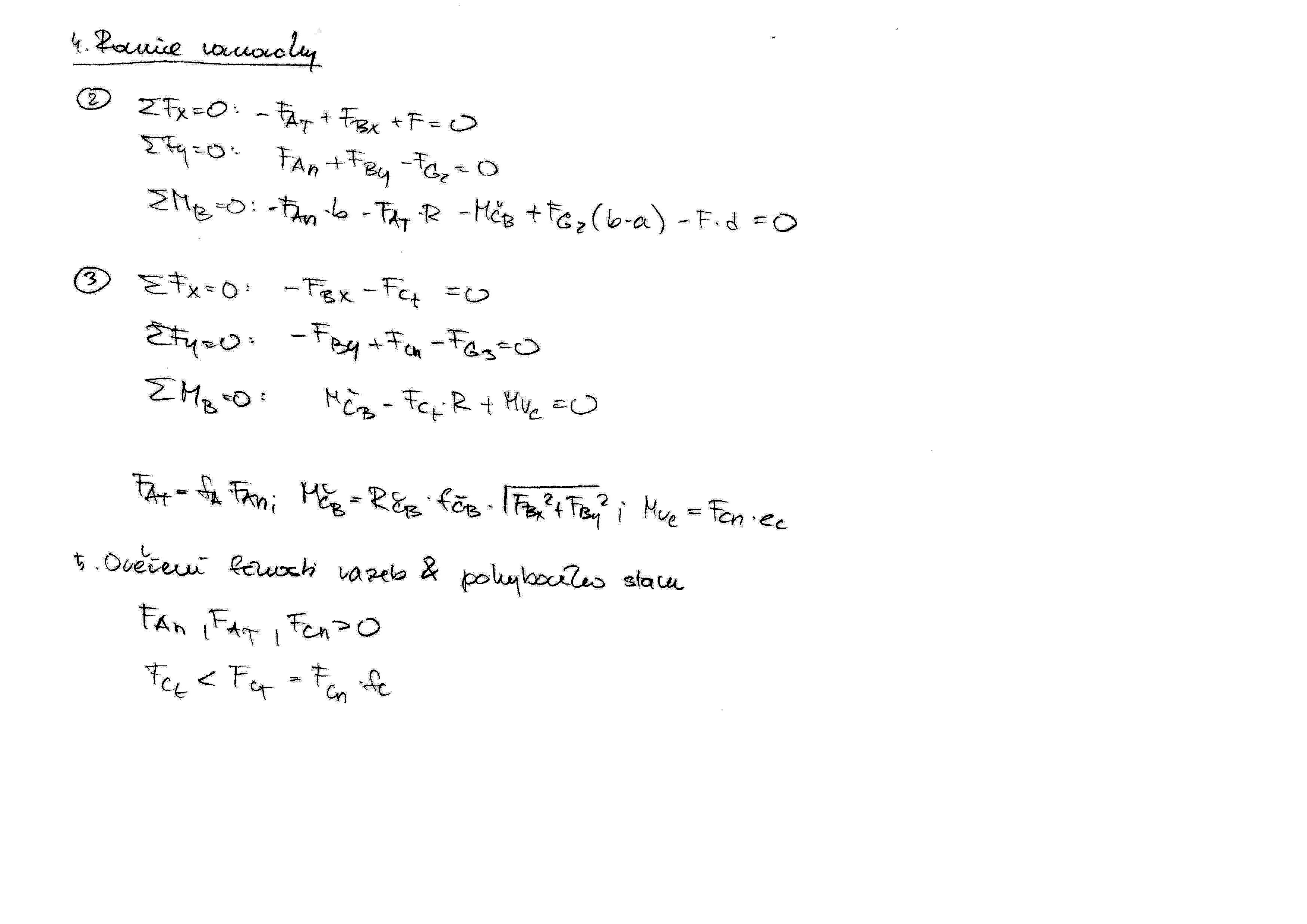
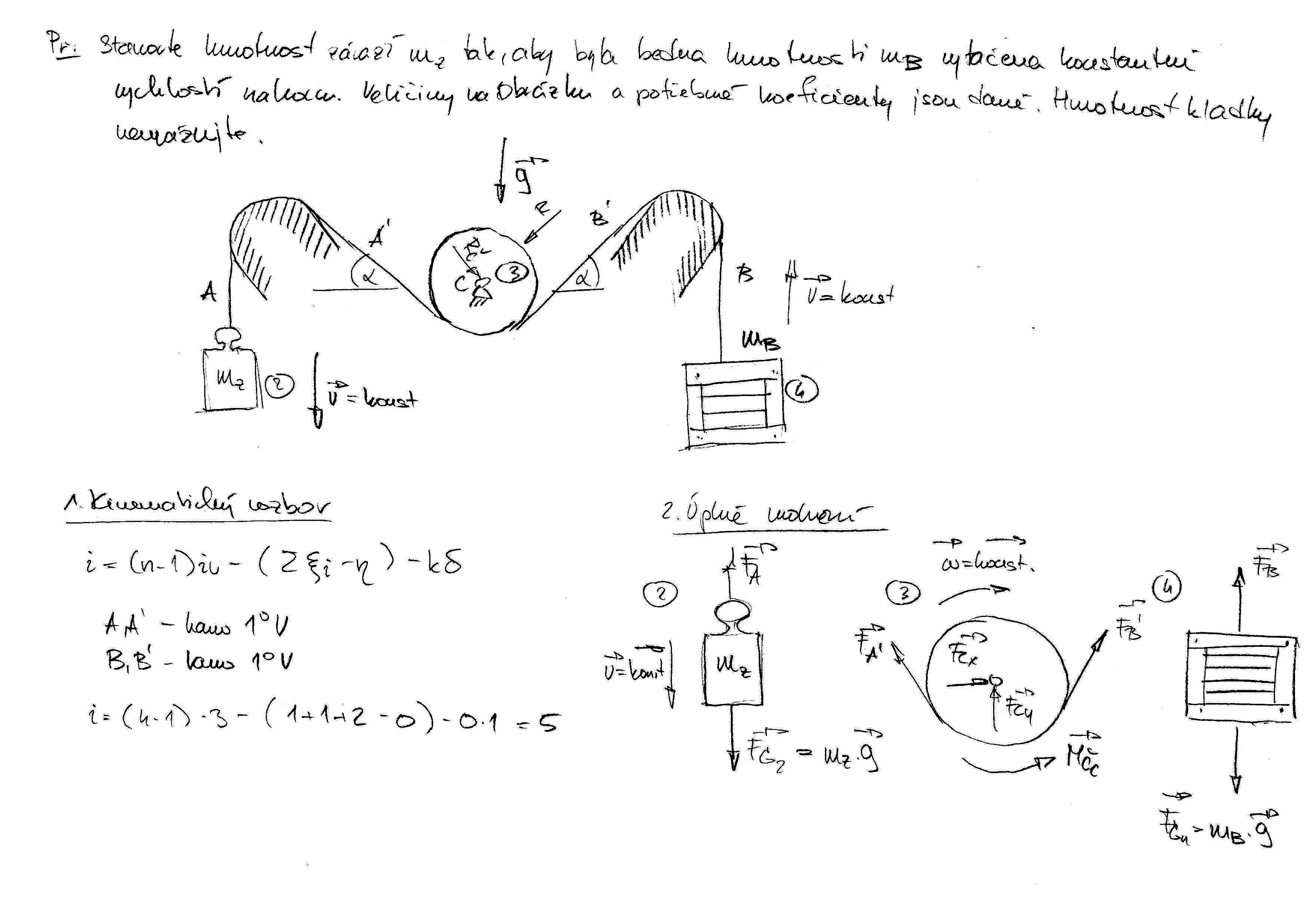
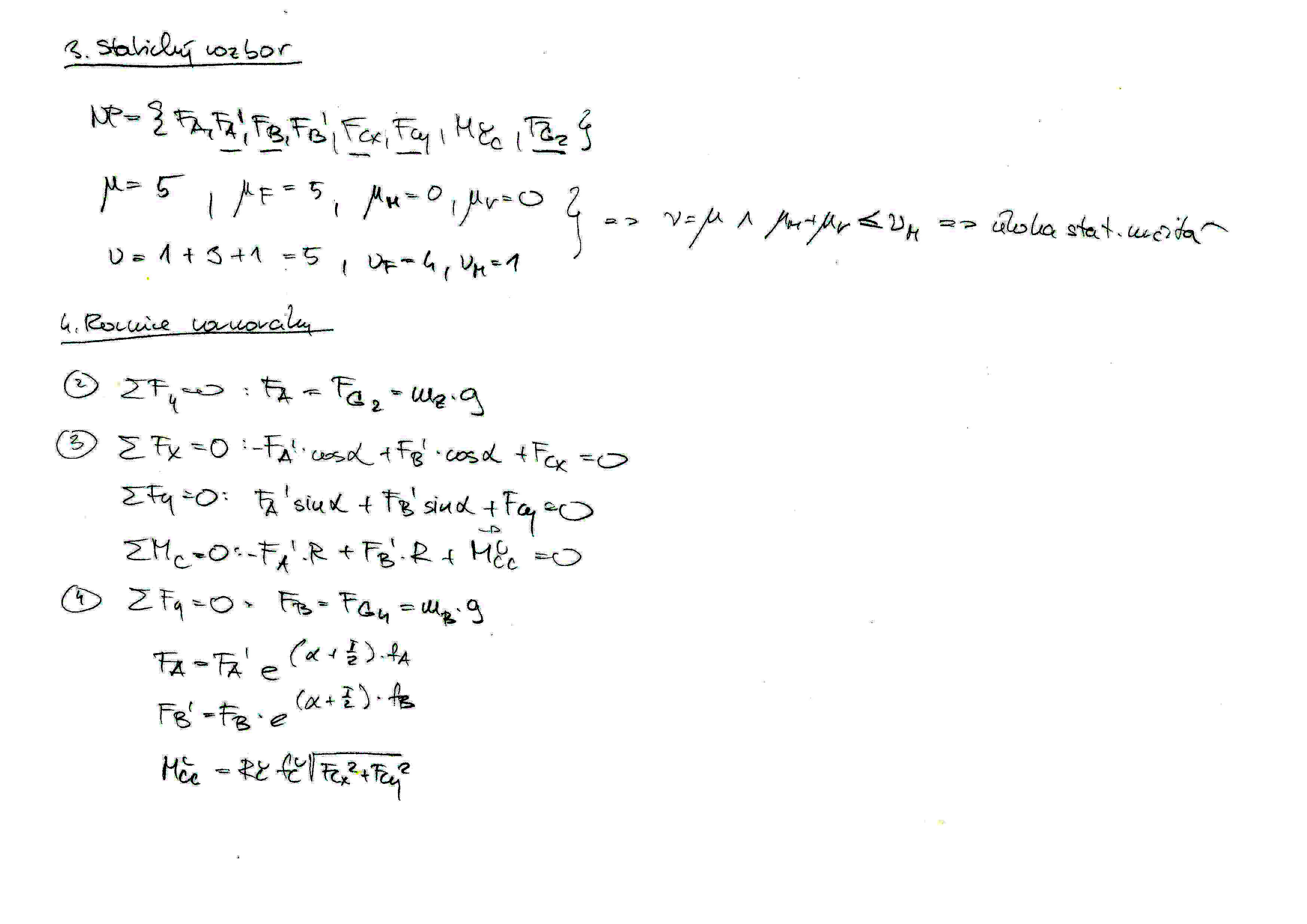
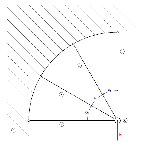
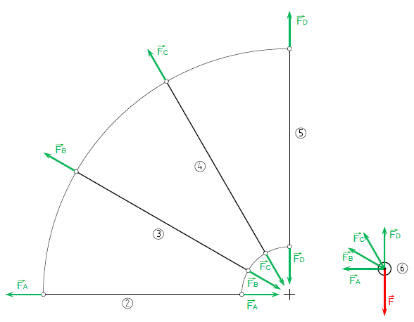
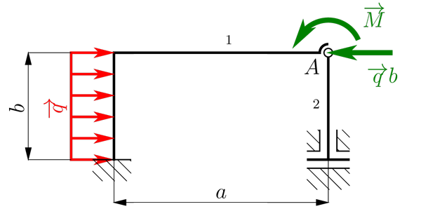
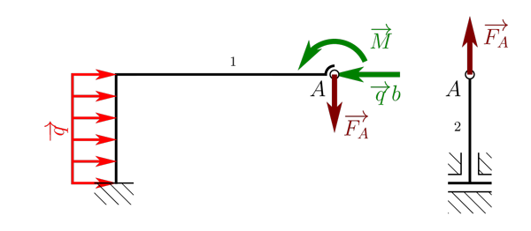
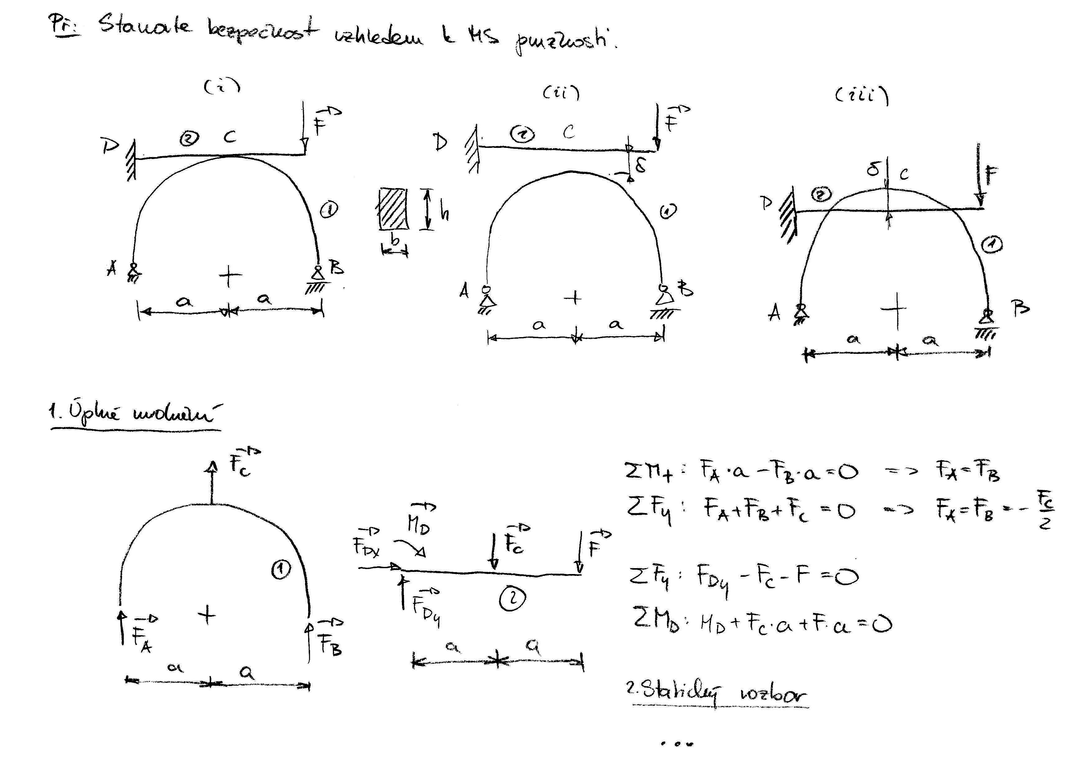
  • Cvičení 1: Síla, moment k bodu, moment k ose.

    • Ručně řešený příklad Př.1 lze stáhnout zde.

    • Ručně řešený příklad Př.2 lze stáhnout zde a zde.

    • Ručně řešený příklad Př.3 lze stáhnout zde.

    • Ručně řešený příklad Př.4 lze stáhnout zde a zde.

    • Ručně řešený příklad Př.5 lze stáhnout zde.

    • Pravidlo pravé ruky, obrázek lze stáhnout zde.

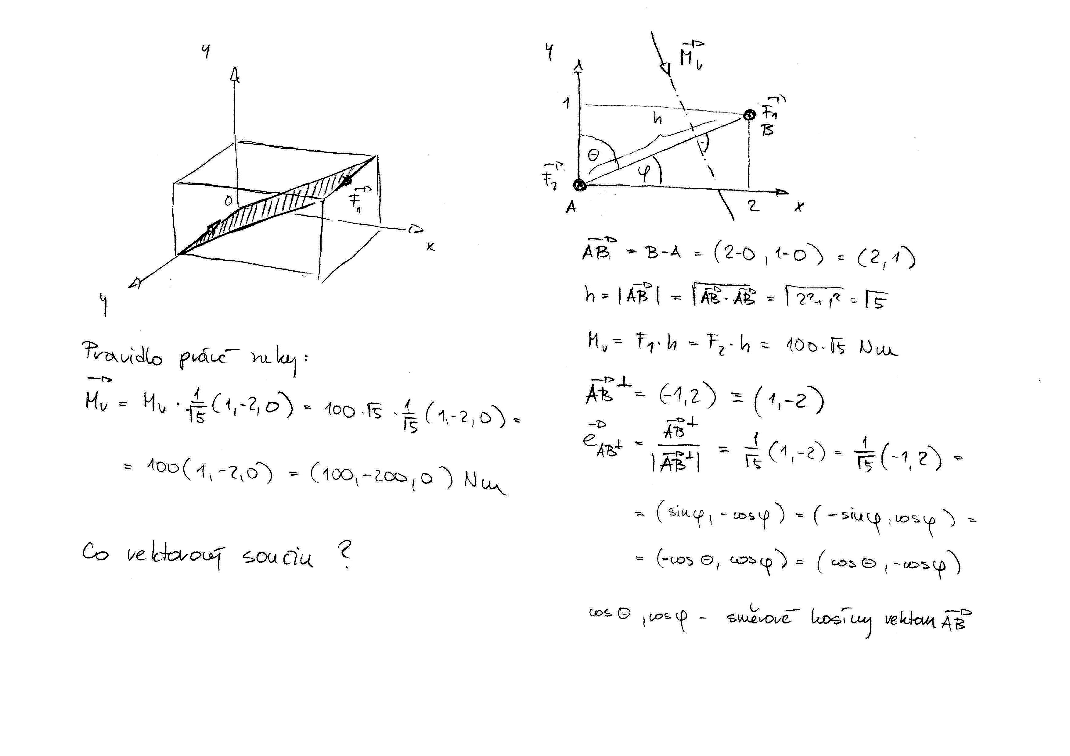
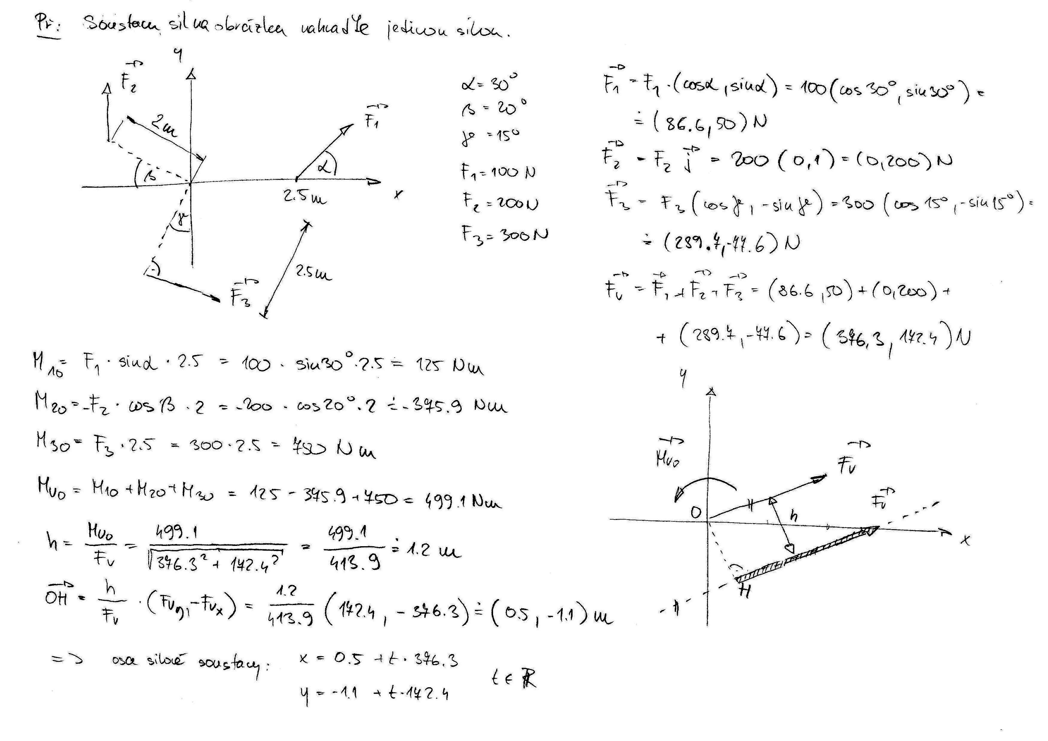
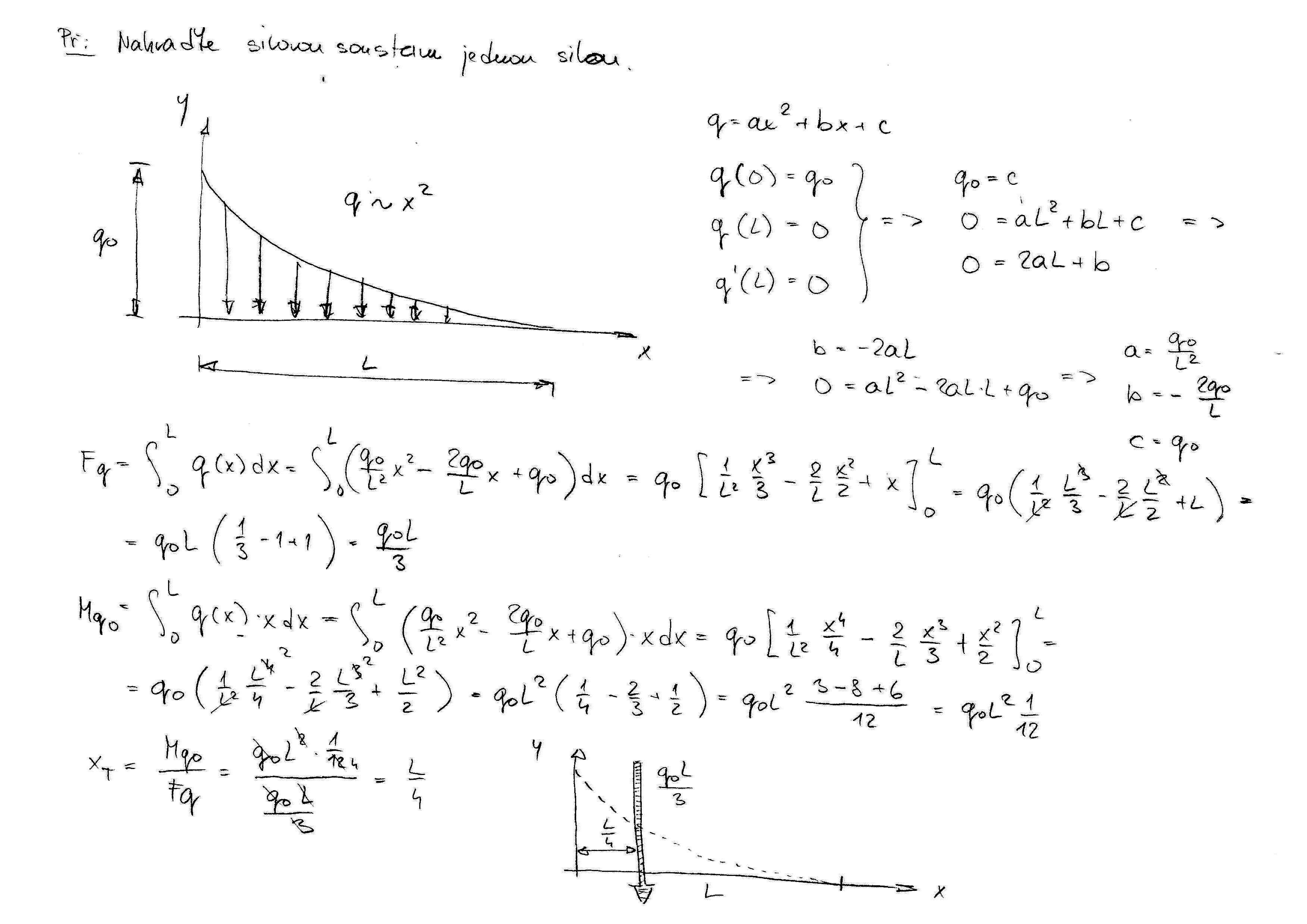
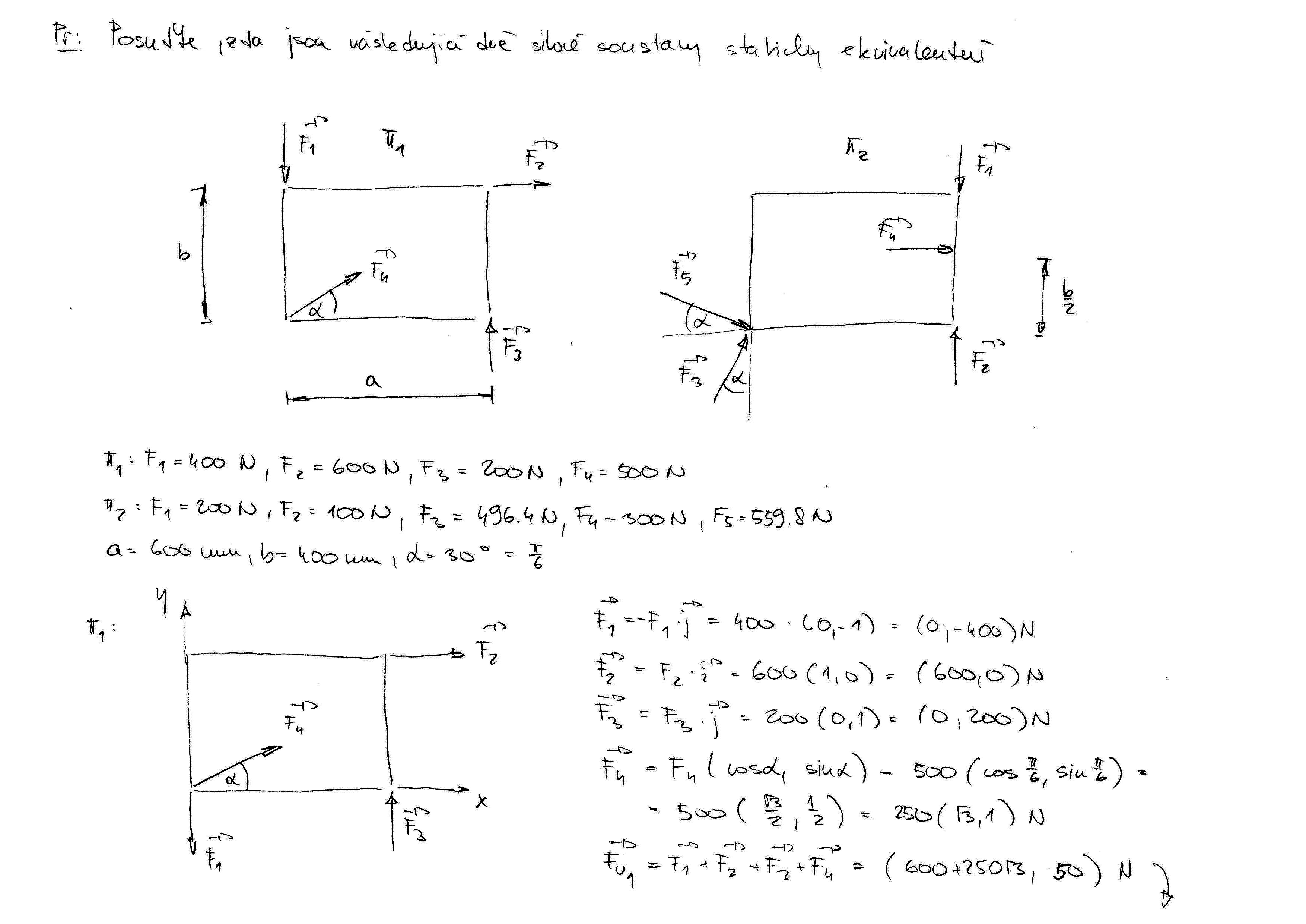
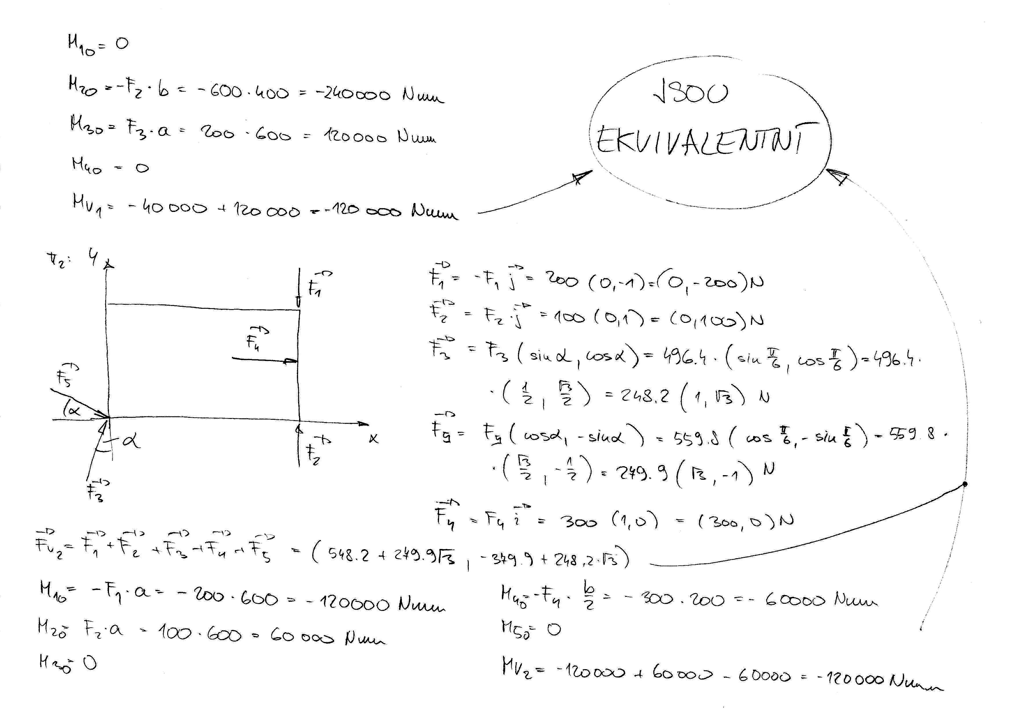
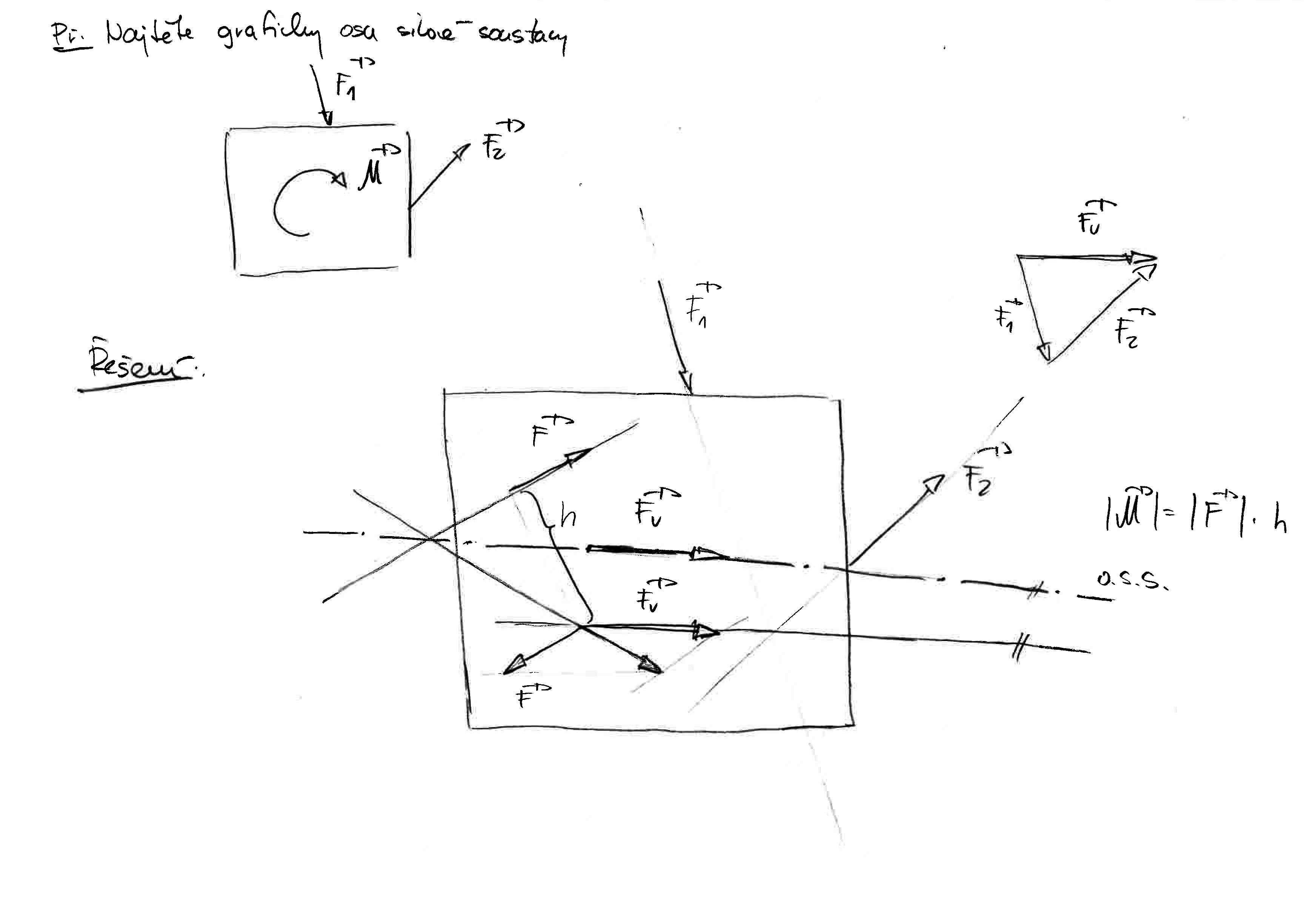
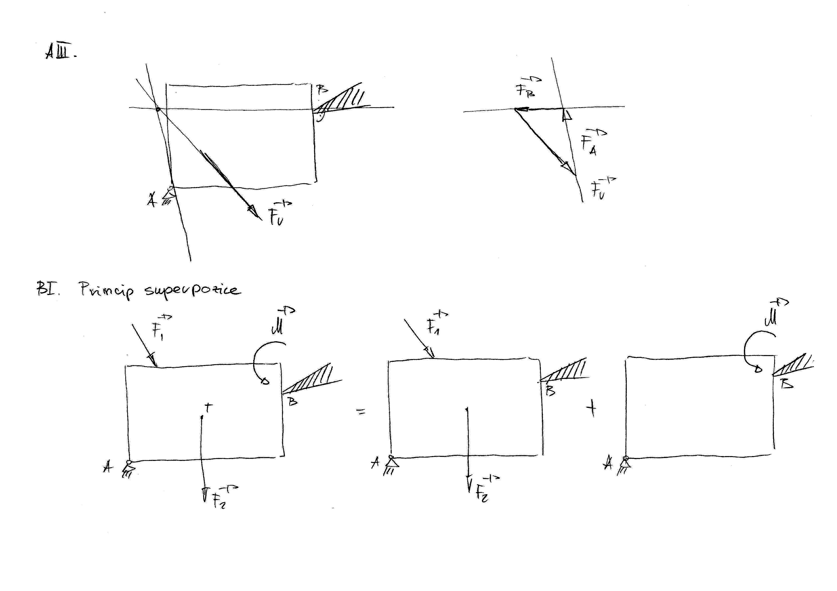
  • Cvičení 2: Silová a momentová výslednice, silová dvojice, osa silové soustavy.

    • Ručně řešený příklad Př.1 lze stáhnout zde a zde.

    • Ručně řešený příklad Př.2 lze stáhnout zde

    • Ručně řešený příklad Př.3 lze stáhnout zde.

    • Ručně řešený příklad Př.4 lze stáhnout zde a zde.

    • Ručně řešený příklad Př.5 lze stáhnout zde a zde..

    • Silová dvojice, obrázek lze stáhnout zde.

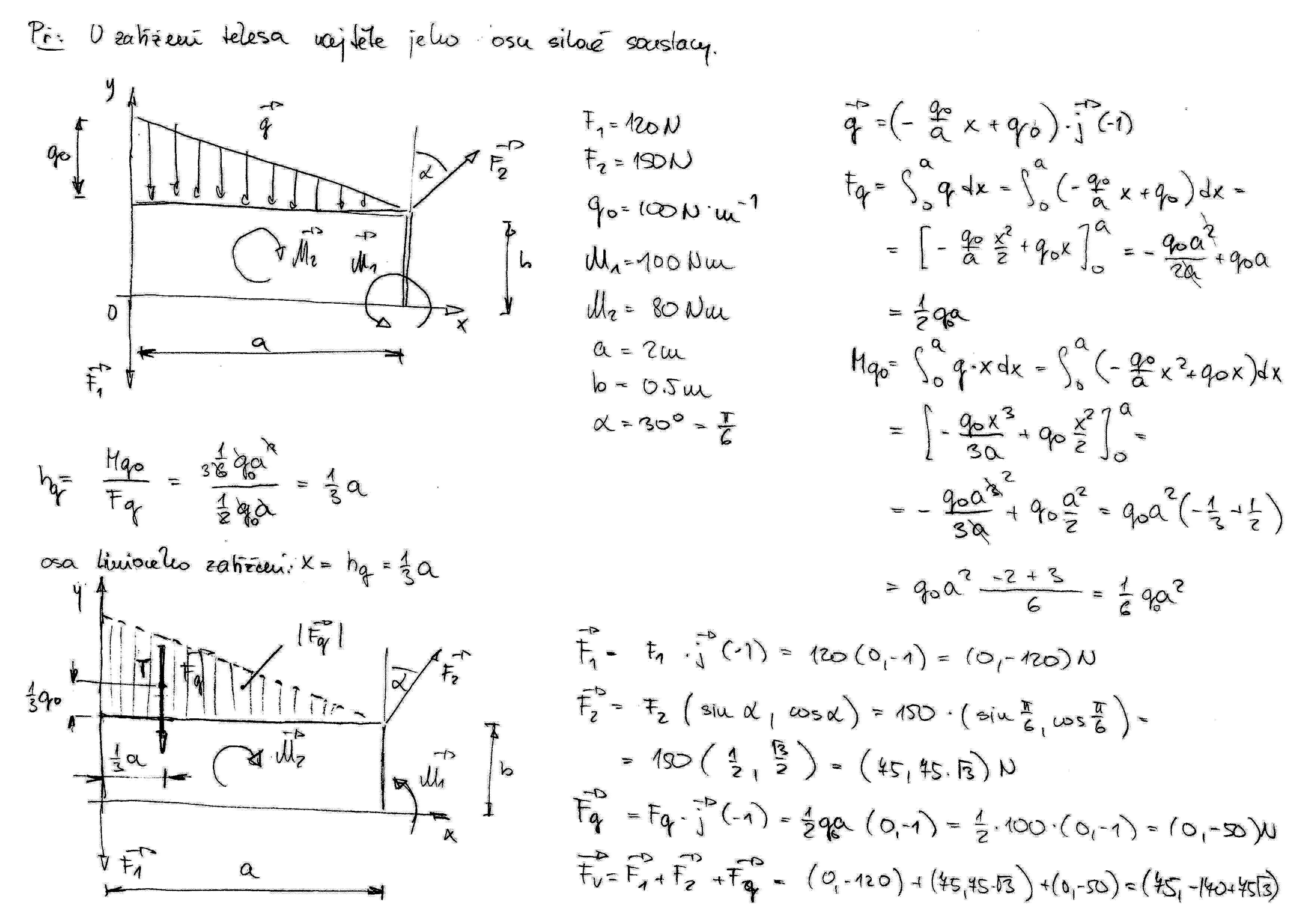
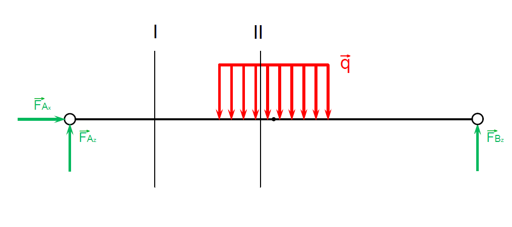
  • Cvičení 3: Osa silové soustavy, liniové zatížení, statická ekvivalence.
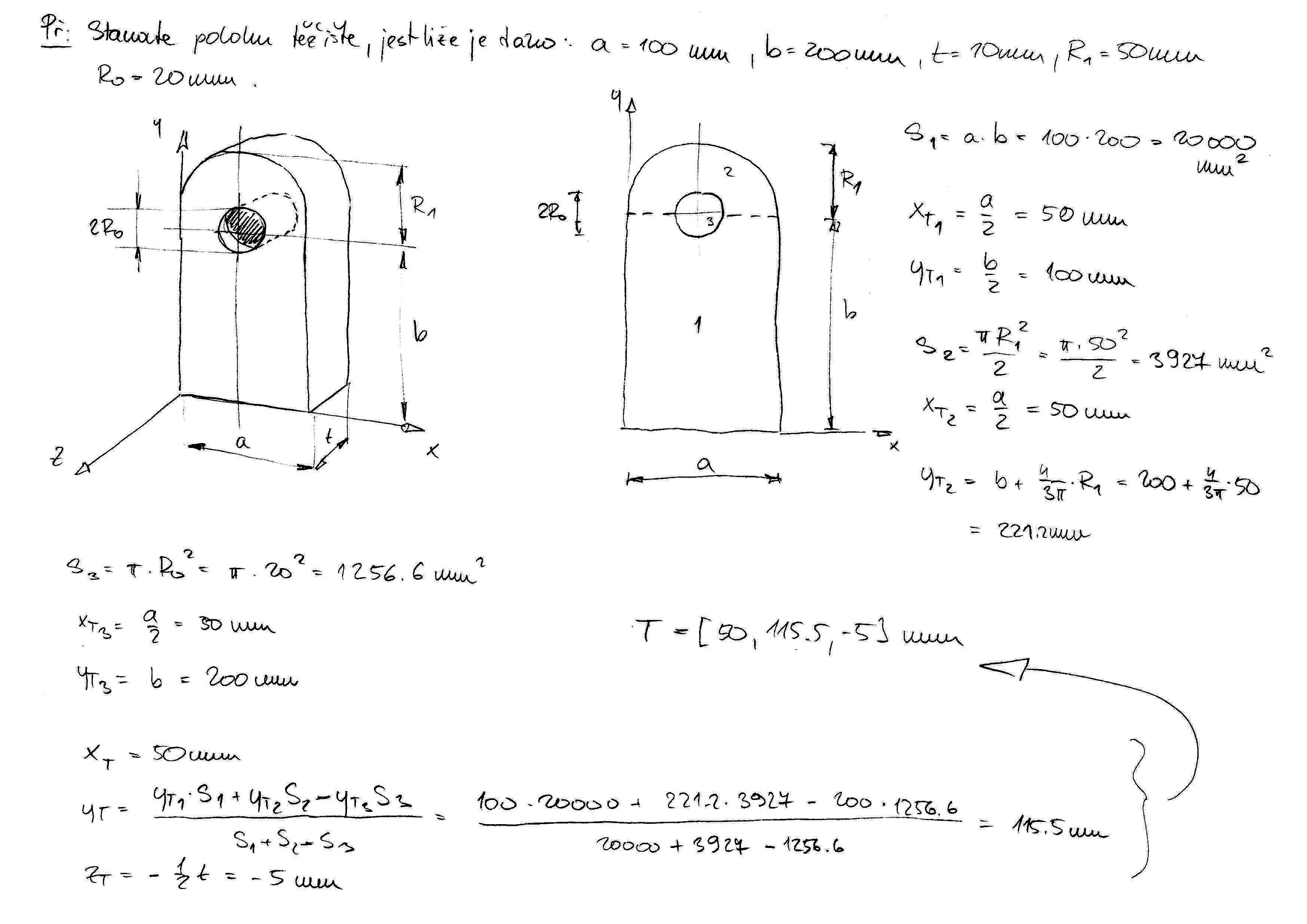
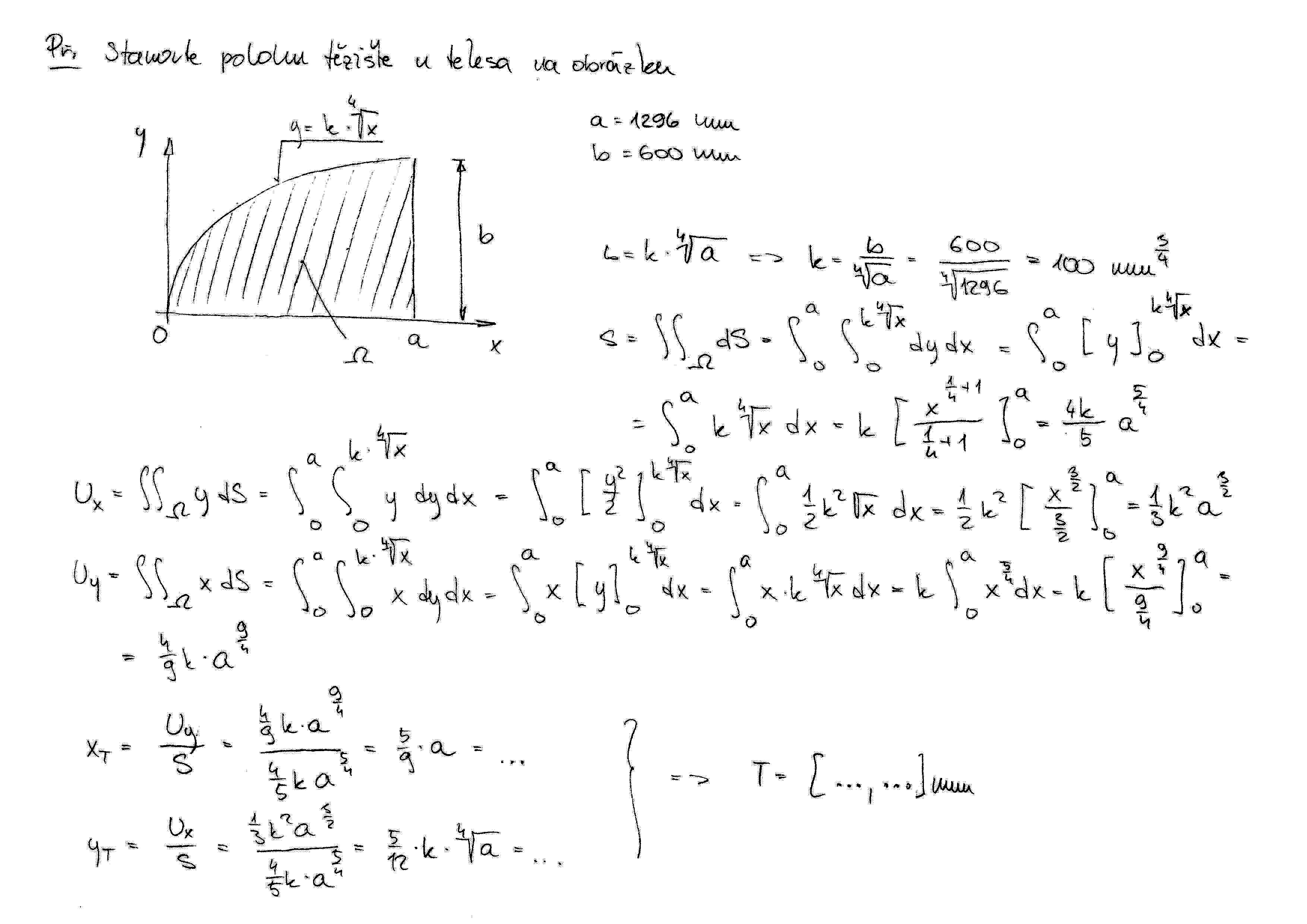
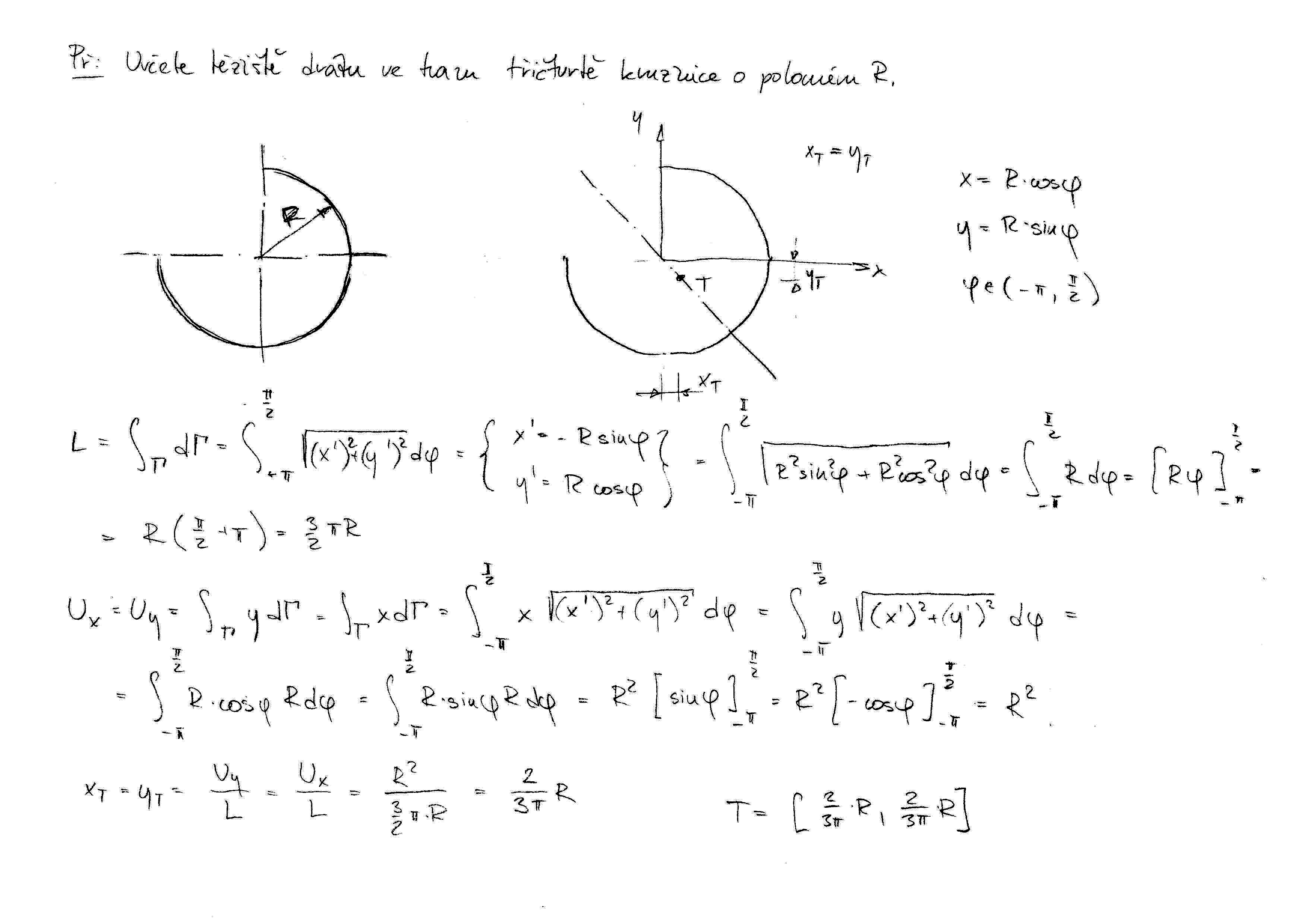
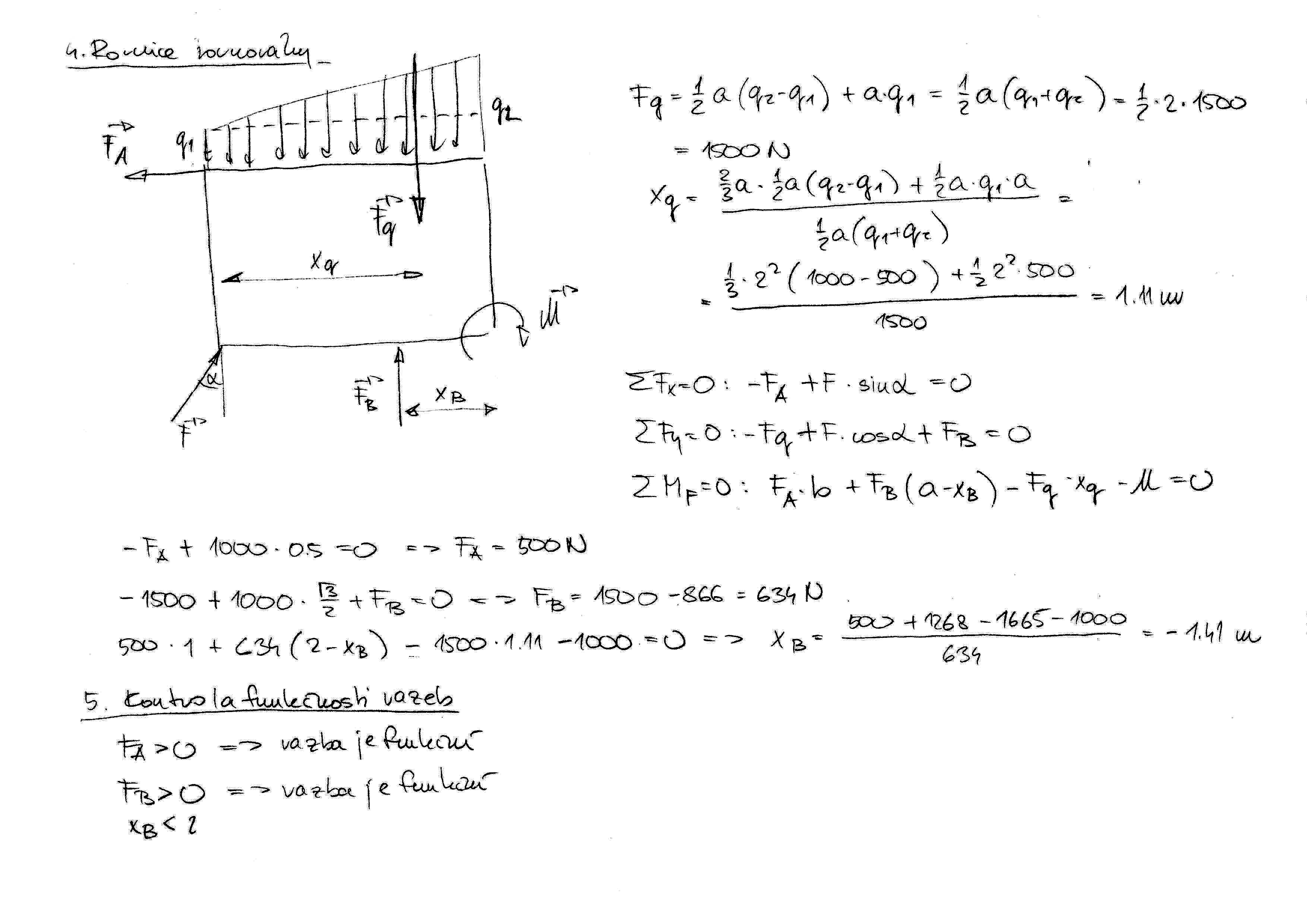
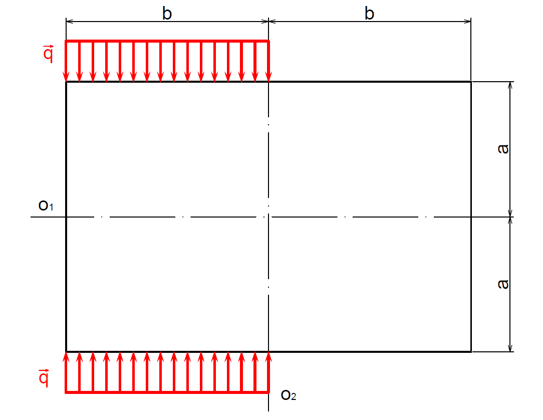
    • Ručně řešený příklad Př.1 lze stáhnout zde.

    • Ručně řešený příklad Př.2 lze stáhnout zde a zde.

    • Ručně řešený příklad Př.3 lze stáhnout zde.

    • Ručně řešený příklad Př.4 lze stáhnout zde a zde.

    • Ručně řešený příklad Př.5 lze stáhnout zde.

    • Liniové zatížení, obrázek lze stáhnout zde.

  • Cvičení 4: Těžiště.

    • Ručně řešený příklad Př.1 lze stáhnout zde.

    • Ručně řešený příklad Př.2 lze stáhnout zde.

    • Ručně řešený příklad Př.3 lze stáhnout zde.

    • Ručně řešený příklad Př.4 lze stáhnout zde.

    • Těžiště, obrázek lze stáhnout zde.

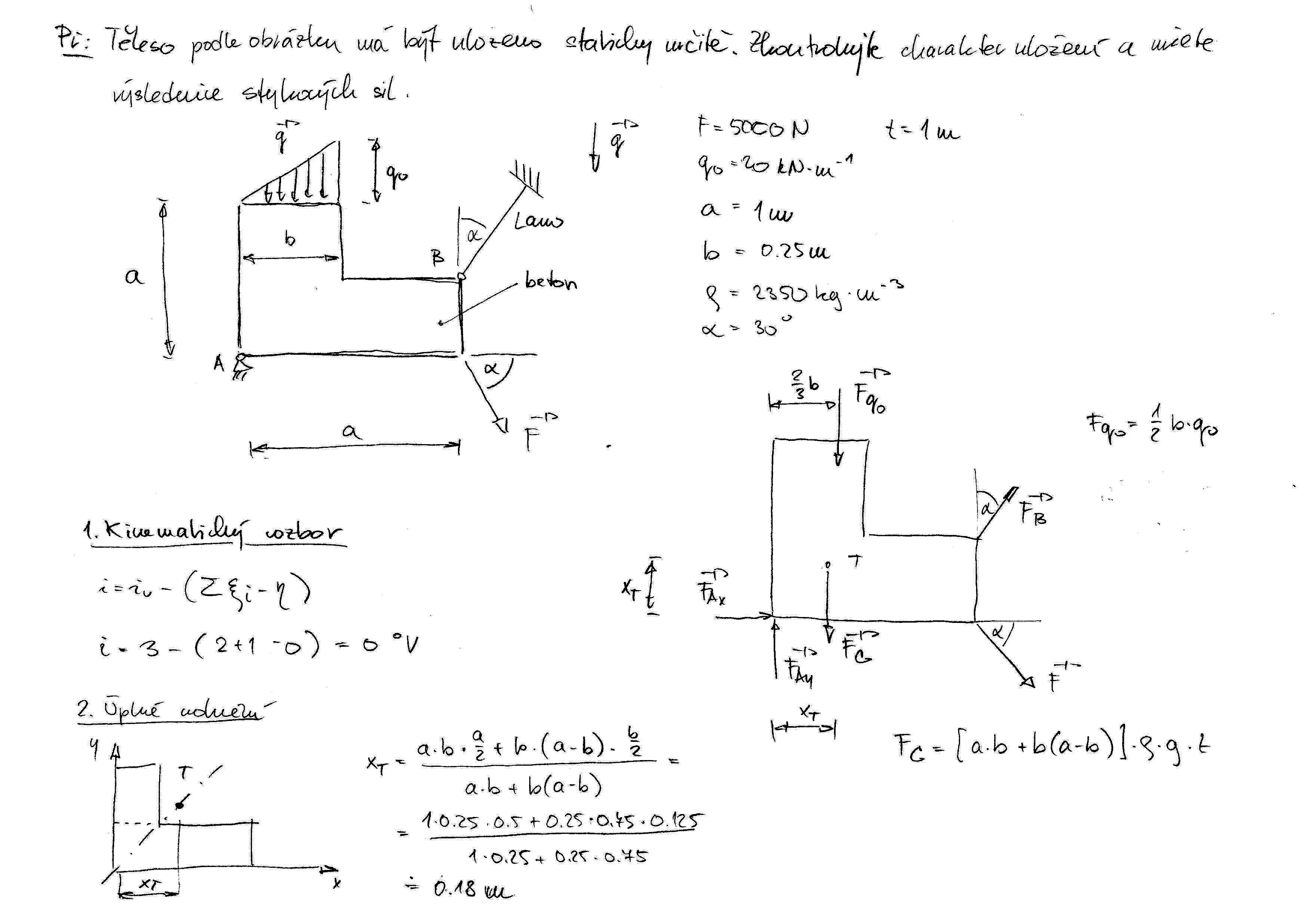
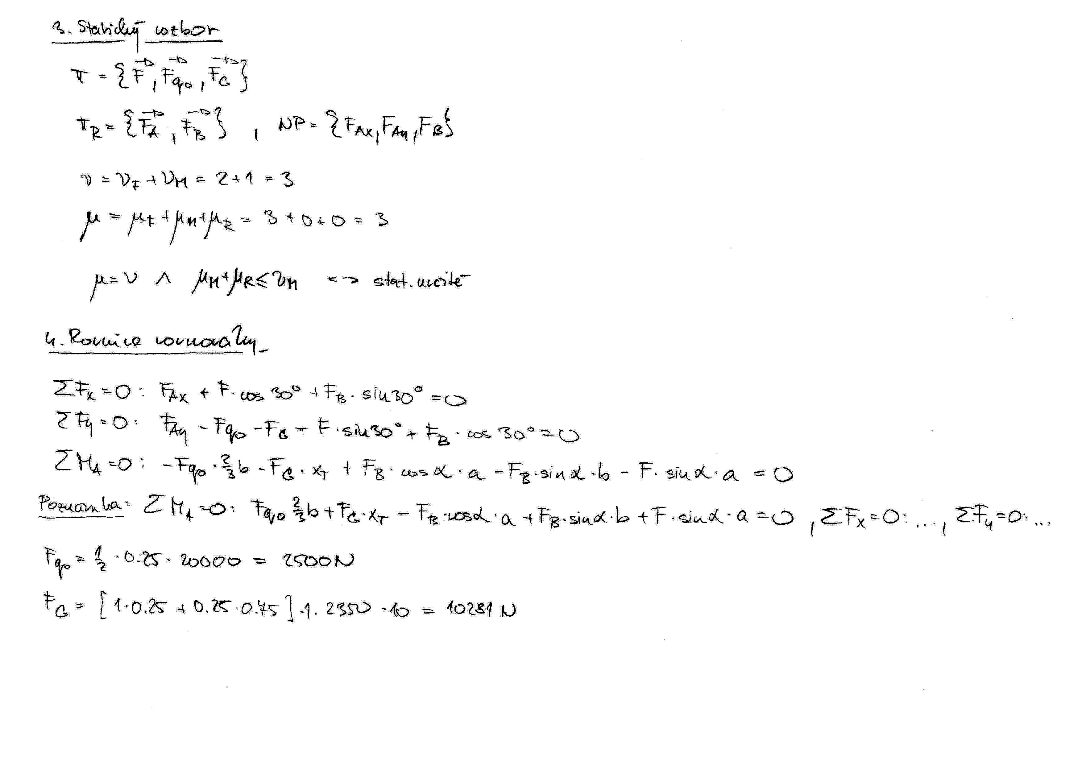
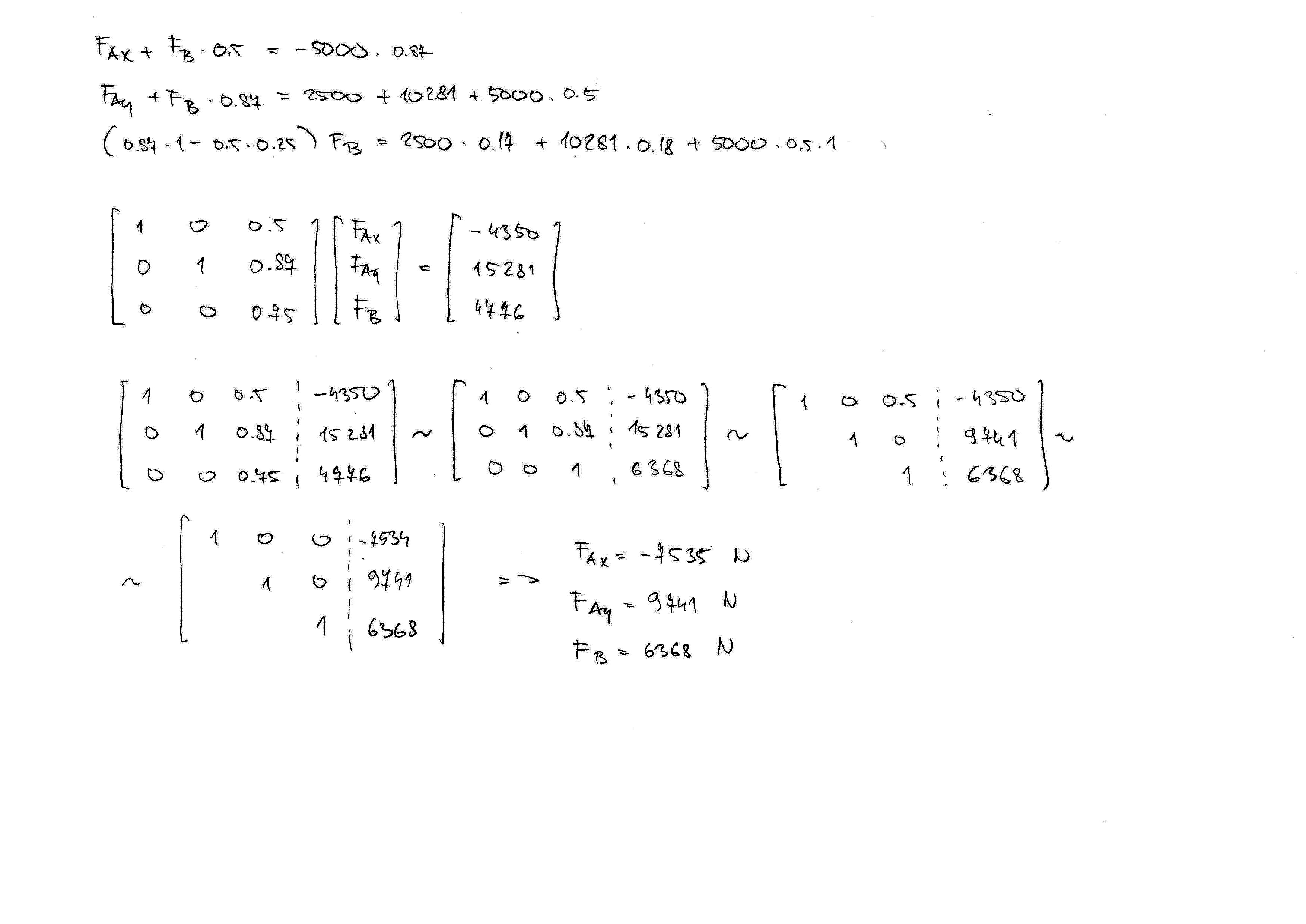
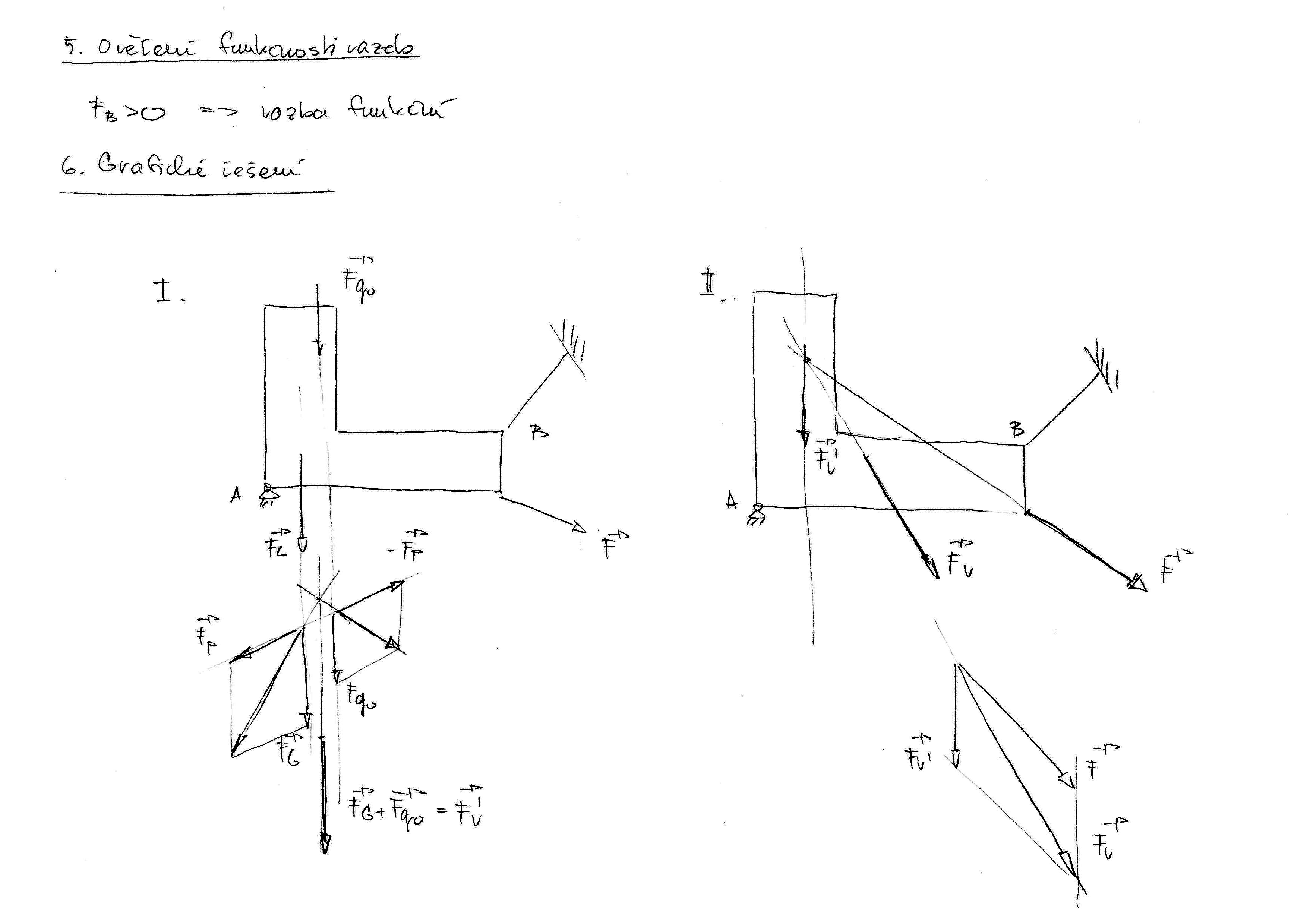
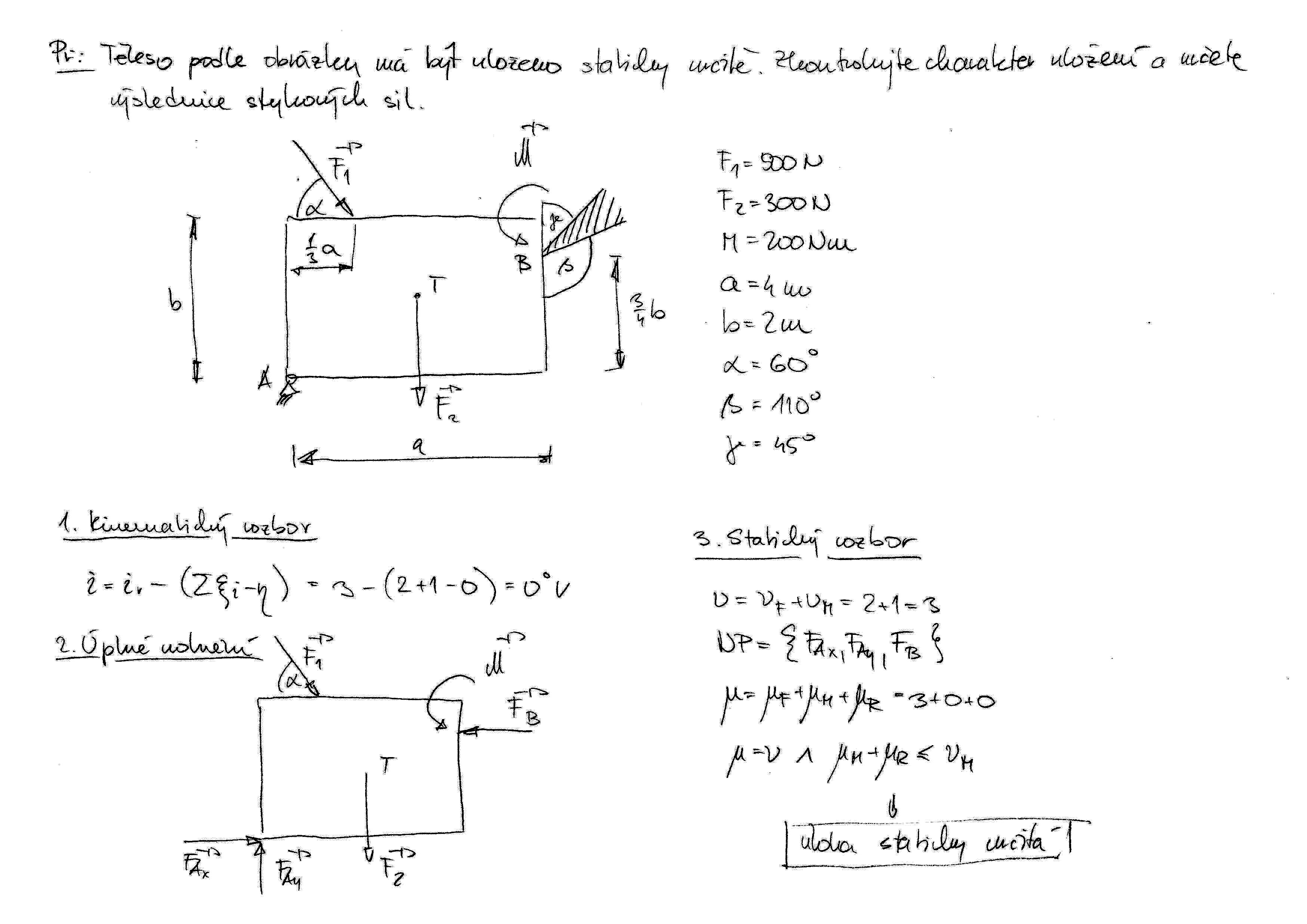
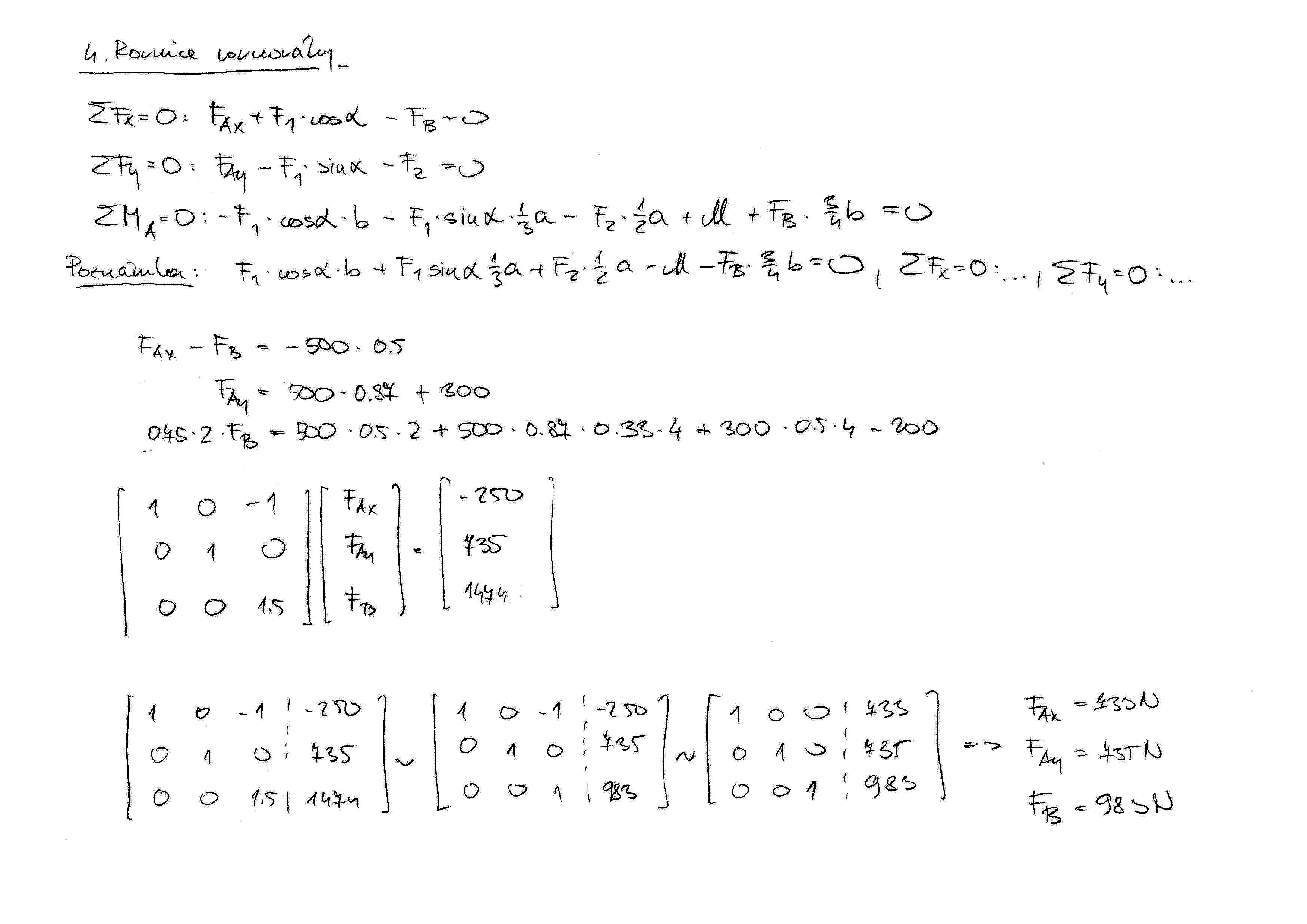
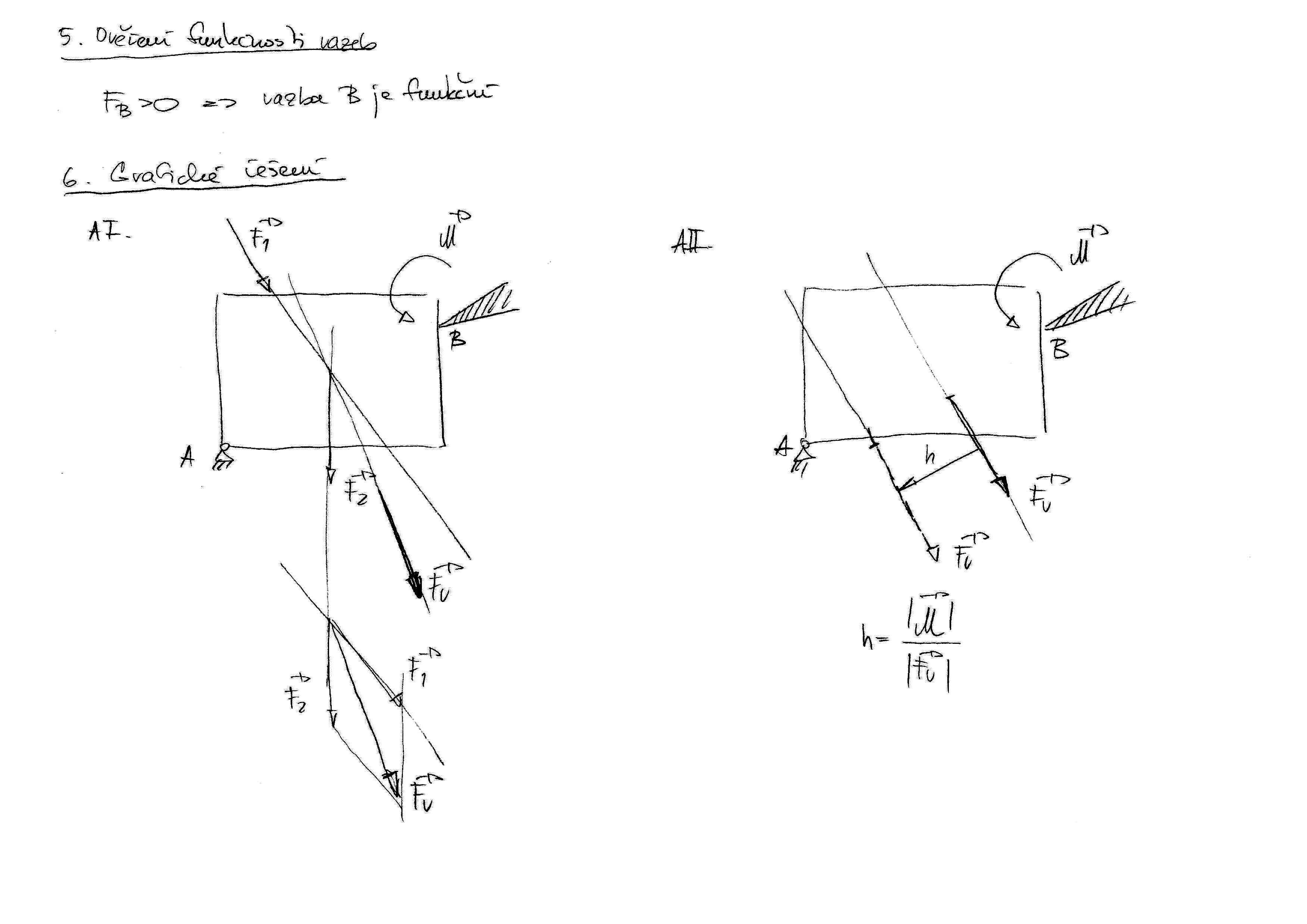
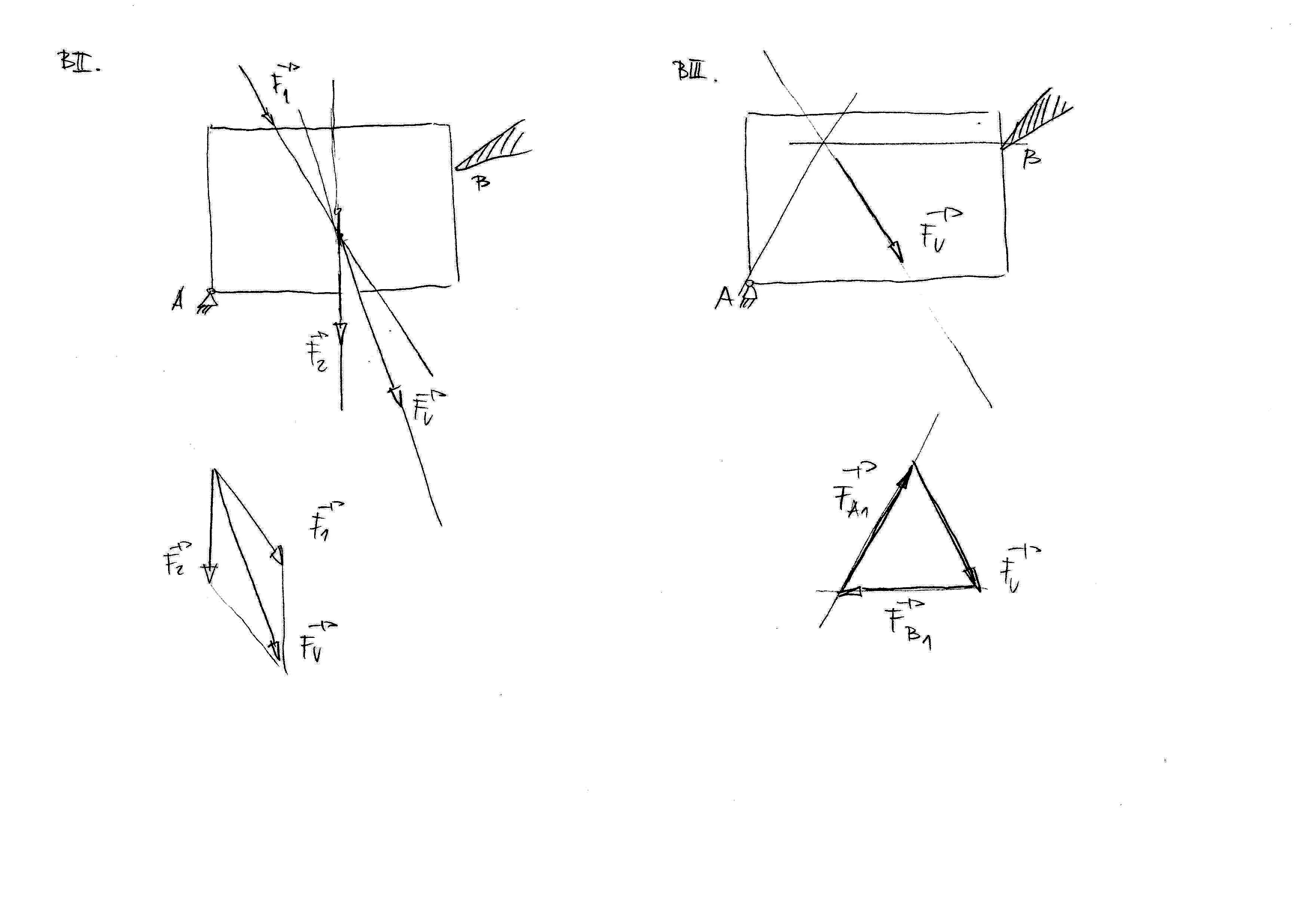
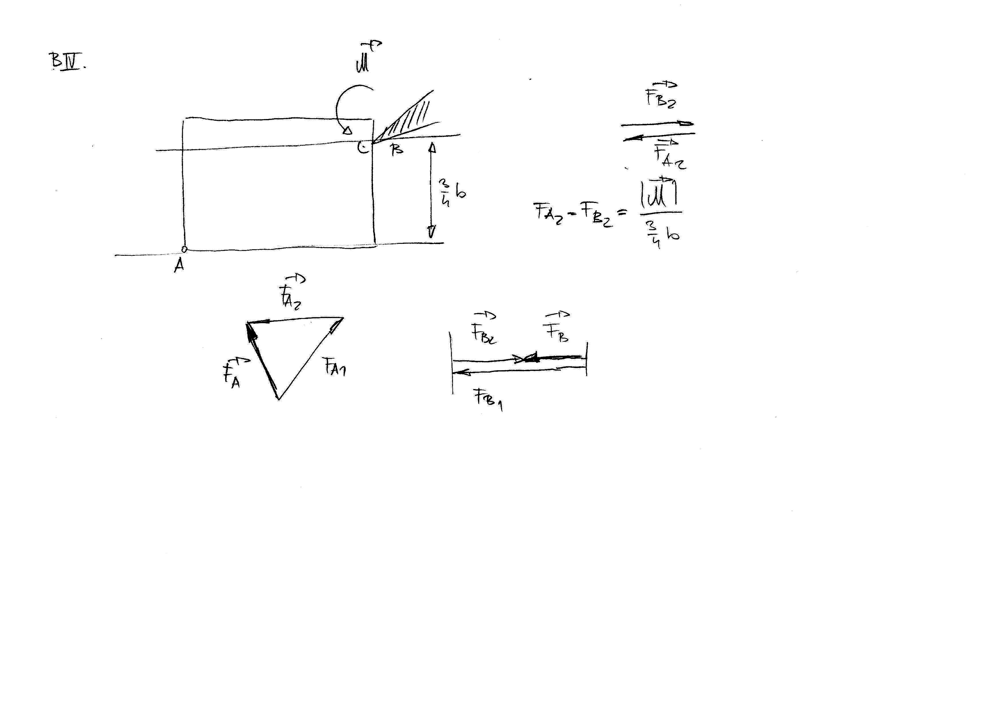
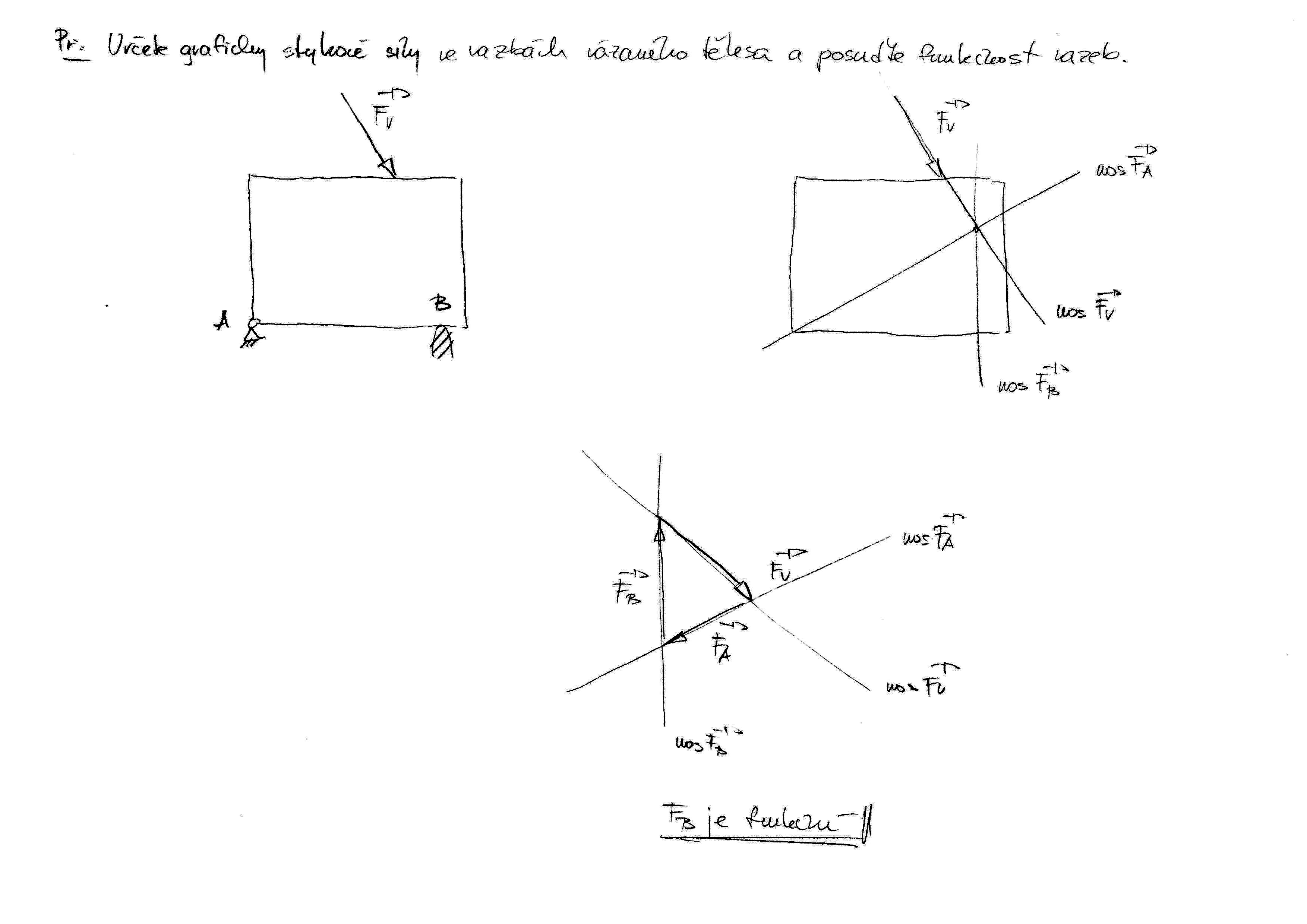
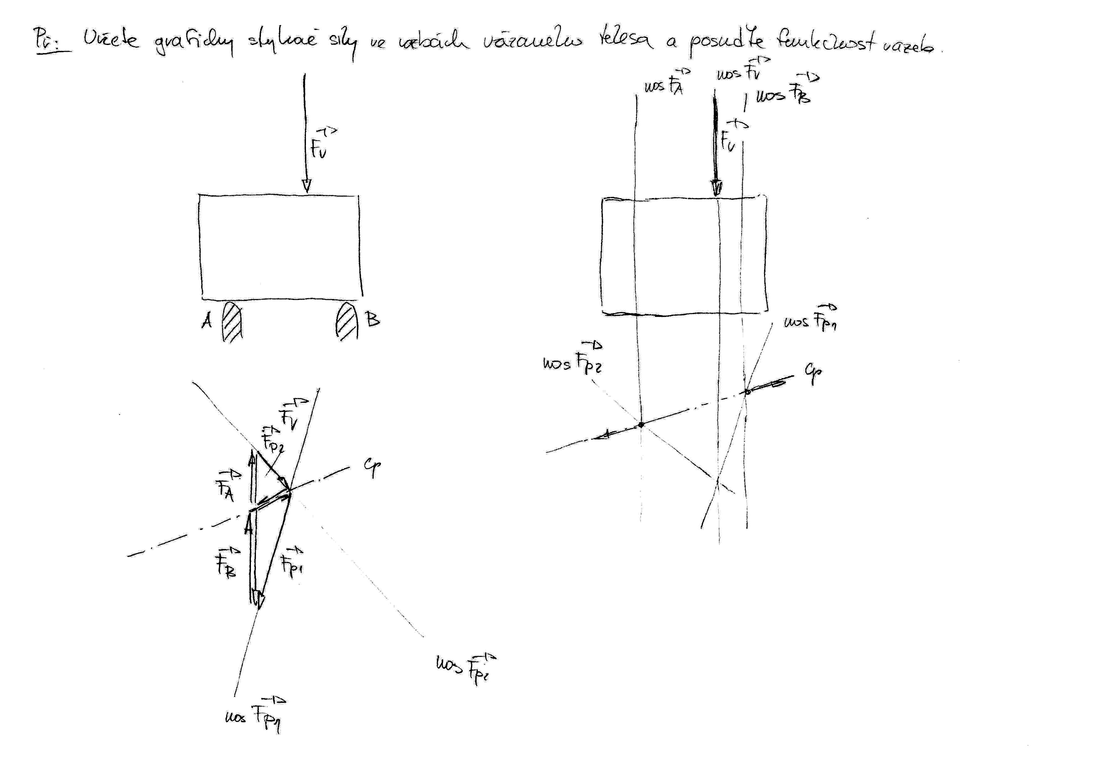
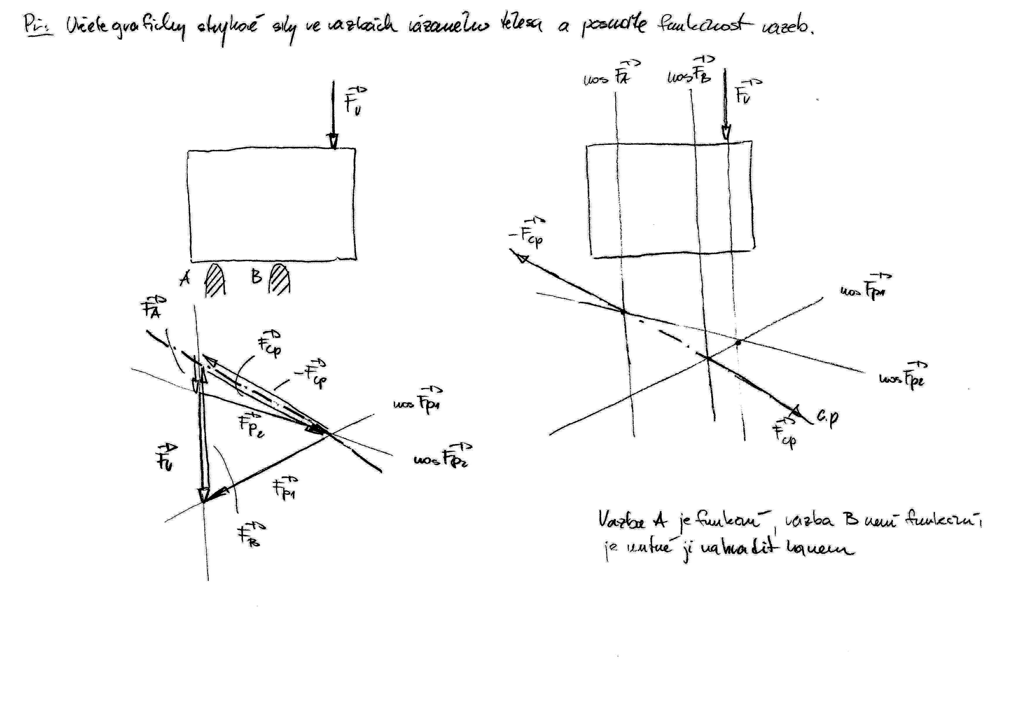
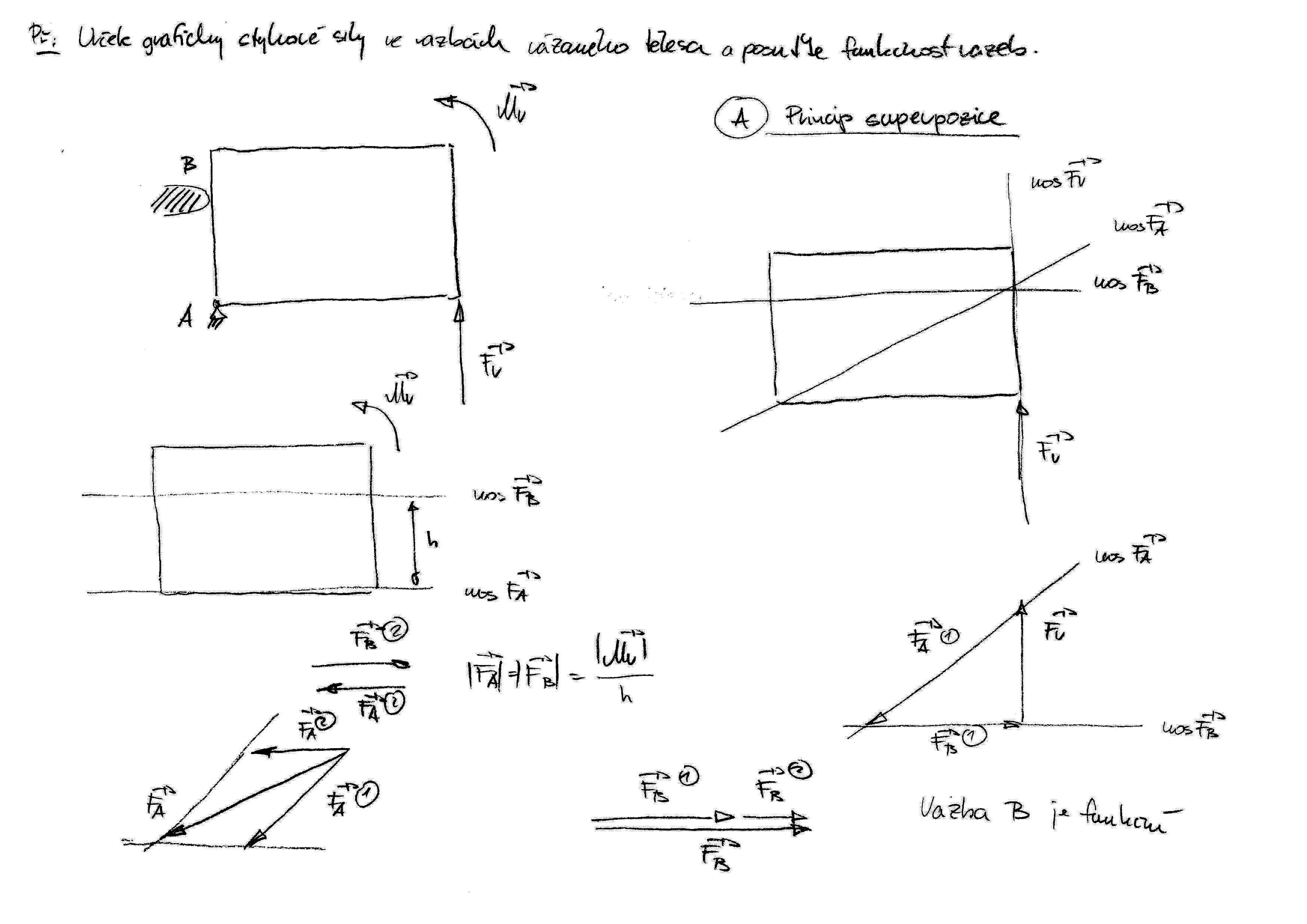
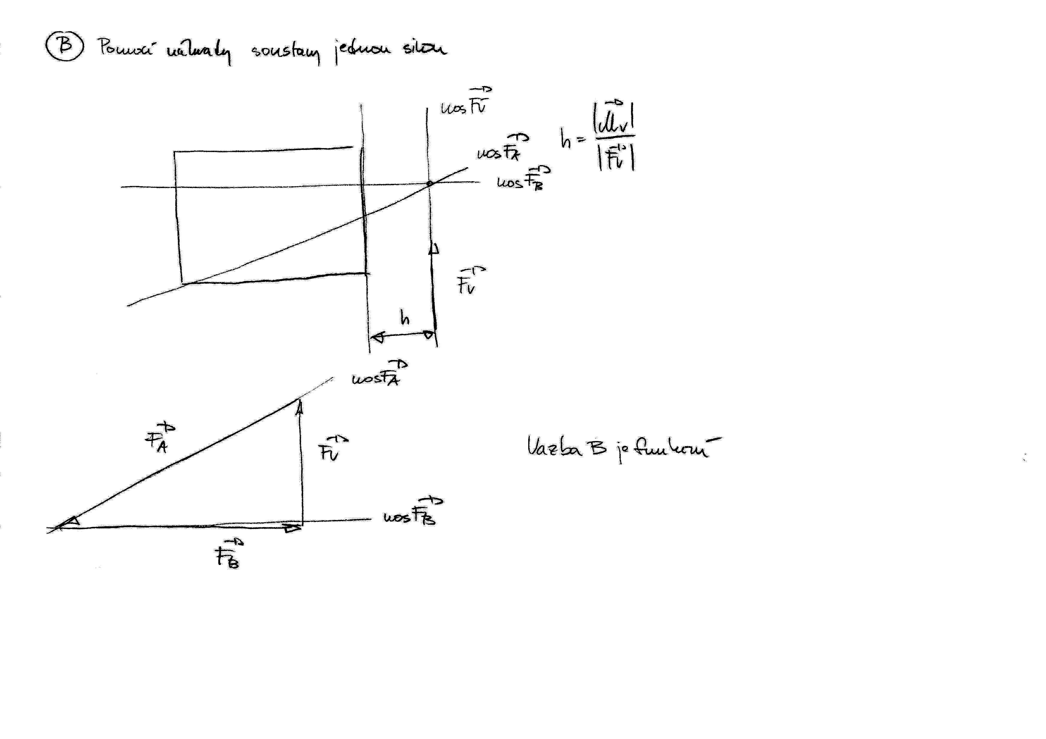
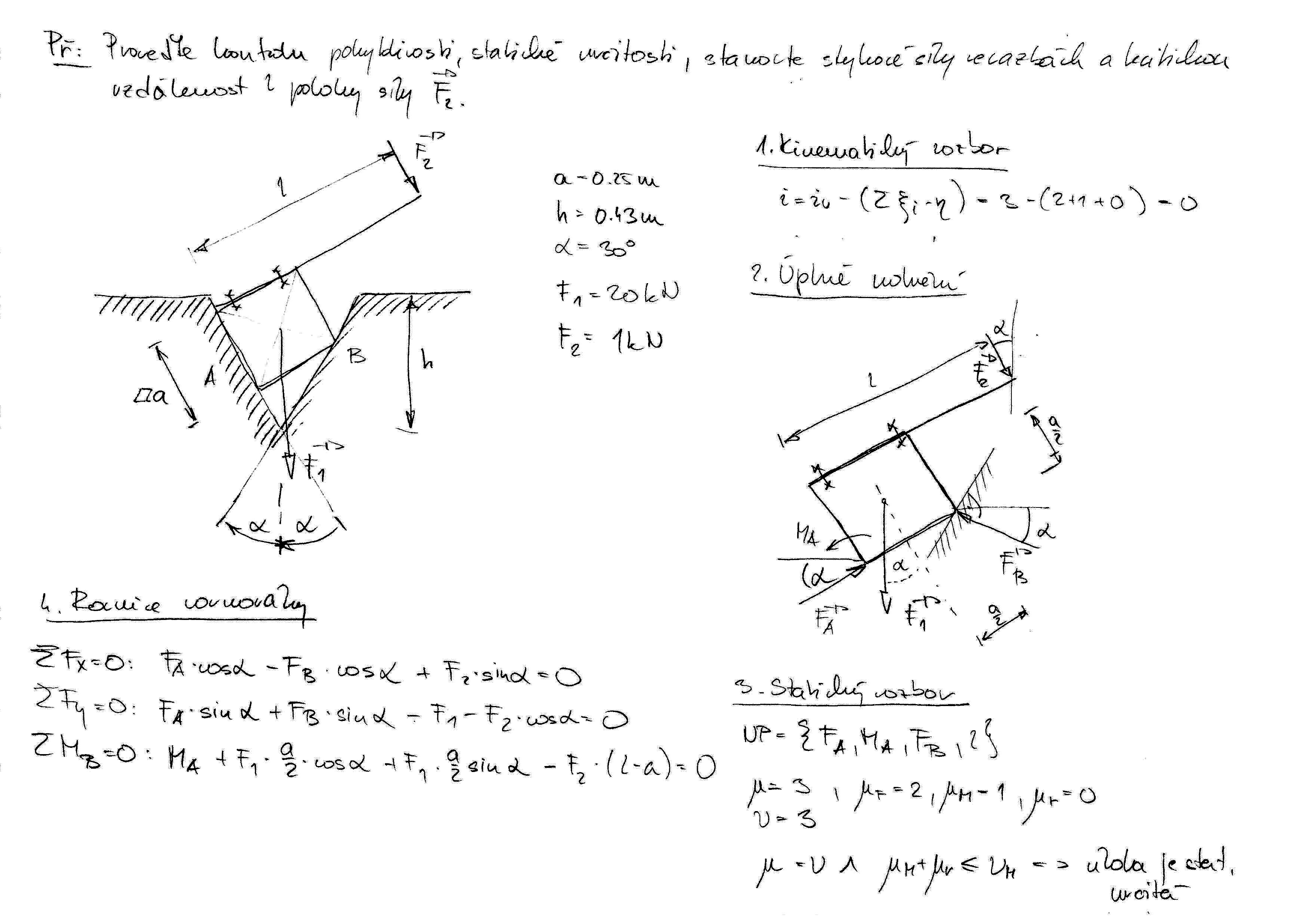
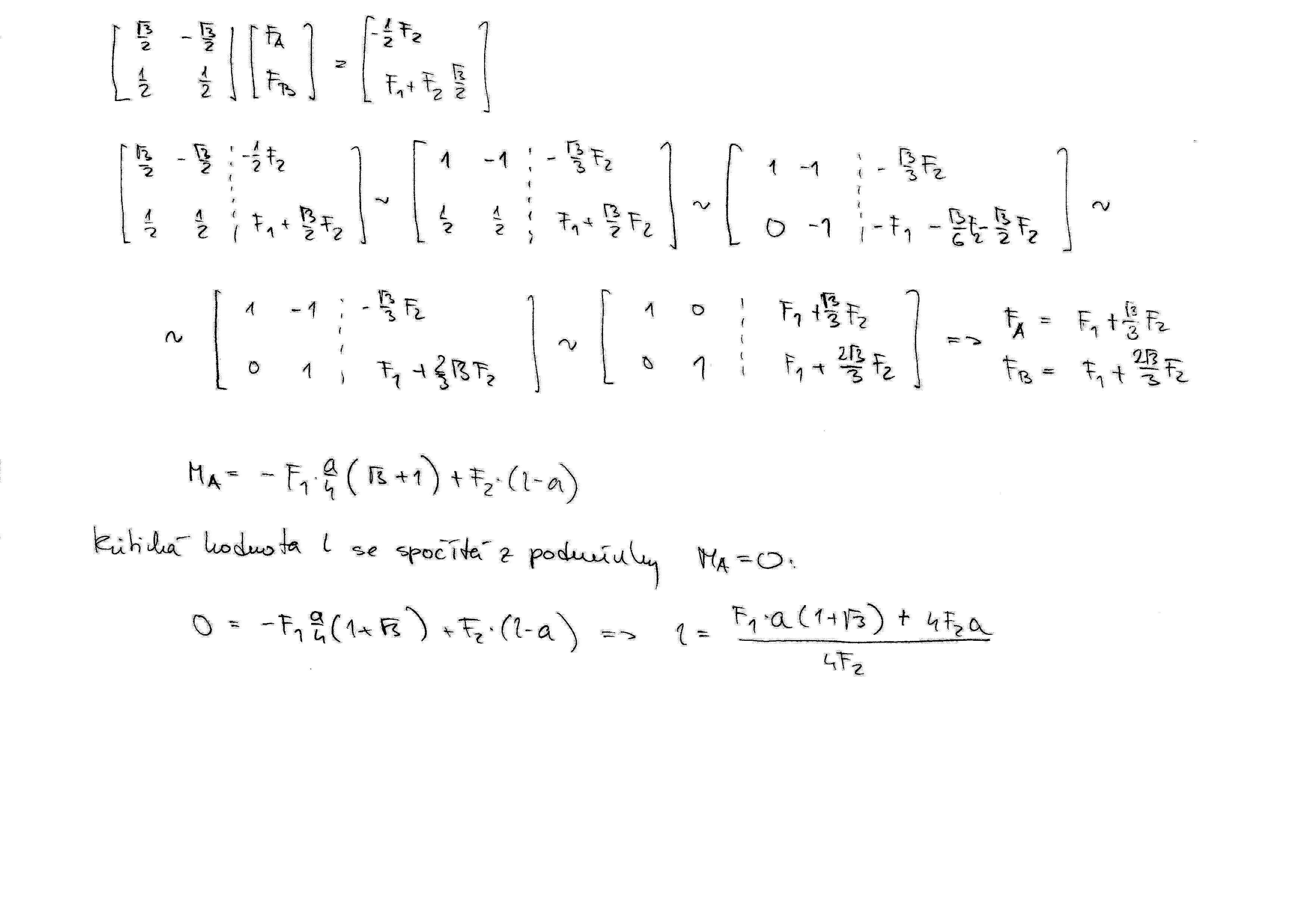
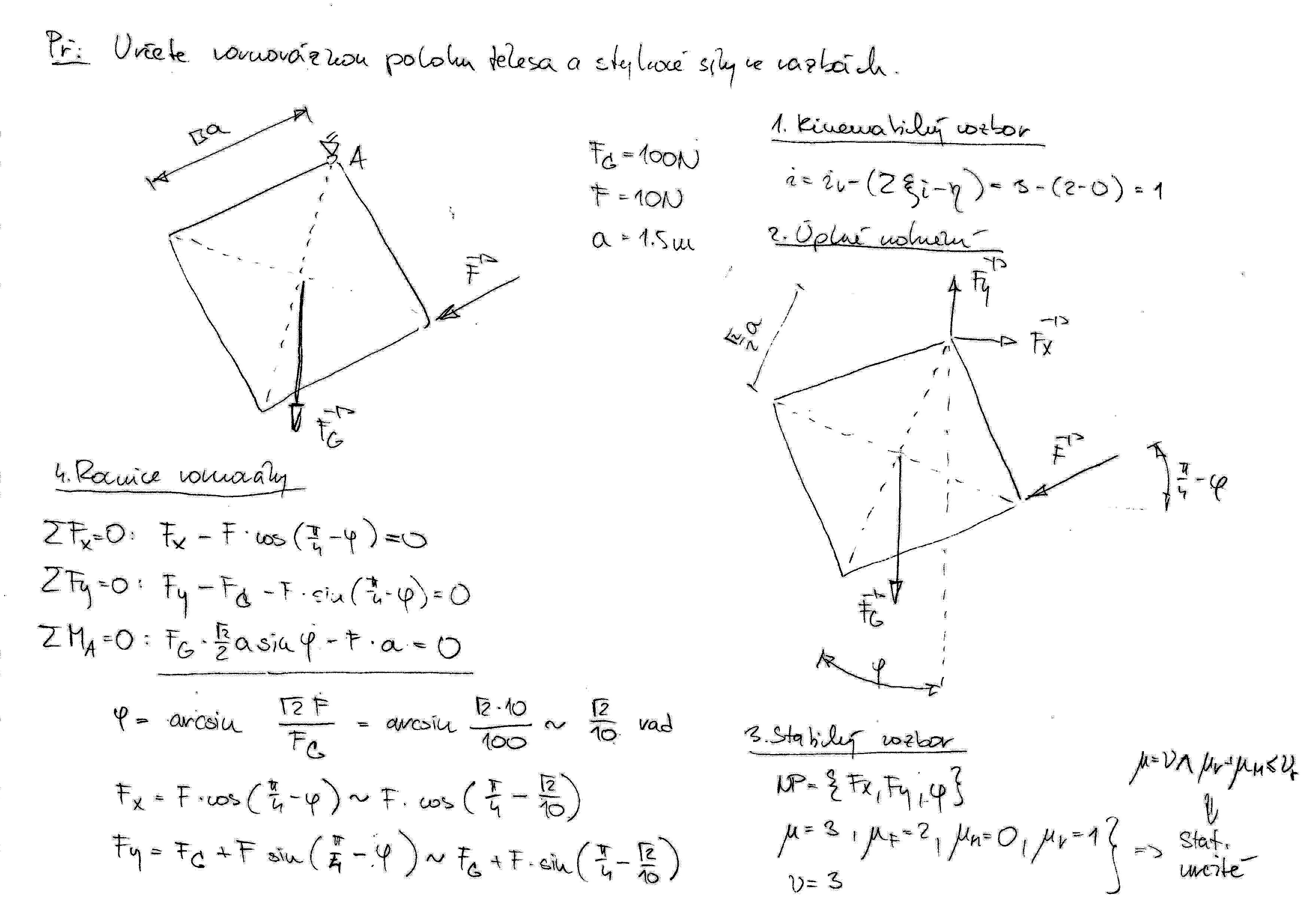
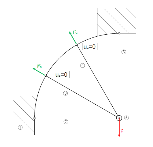
  • Cvičení 5: Vázané těleso.

    • Ručně řešený příklad Př.1 lze stáhnout zde, zde, zde, zde a zde.

    • Ručně řešený příklad Př.2 lze stáhnout zde, zde, zde, zde, zde a zde.

    • Ručně řešený příklad Př.3 lze stáhnout zde, zde, zde a zde.

    • Vazby, obrázek lze stáhnout zde.

  • Cvičení 6: Vázané těleso.

    • Ručně řešený příklad Př.1 lze stáhnout zde.

    • Ručně řešený příklad Př.2 lze stáhnout zde.

    • Ručně řešený příklad Př.3 lze stáhnout zde.

    • Ručně řešený příklad Př.4 lze stáhnout zde.

    • Ručně řešený příklad Př.5 lze stáhnout zde.

    • Ručně řešený příklad Př.6 lze stáhnout zde a zde.

    • Ručně řešený příklad Př.7 lze stáhnout zde a zde.

    • Silové obrazce, obrázek lze stáhnout zde.

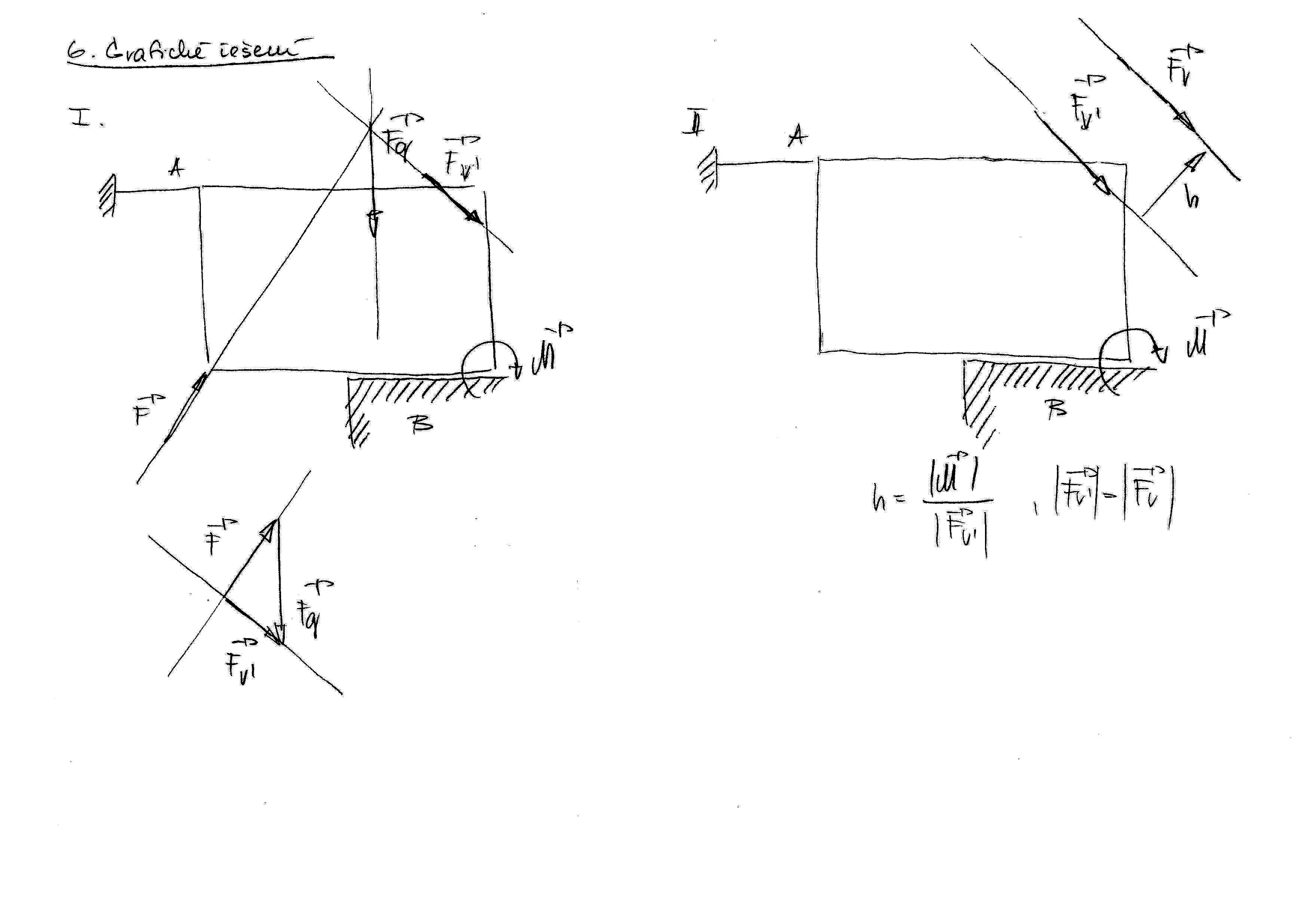
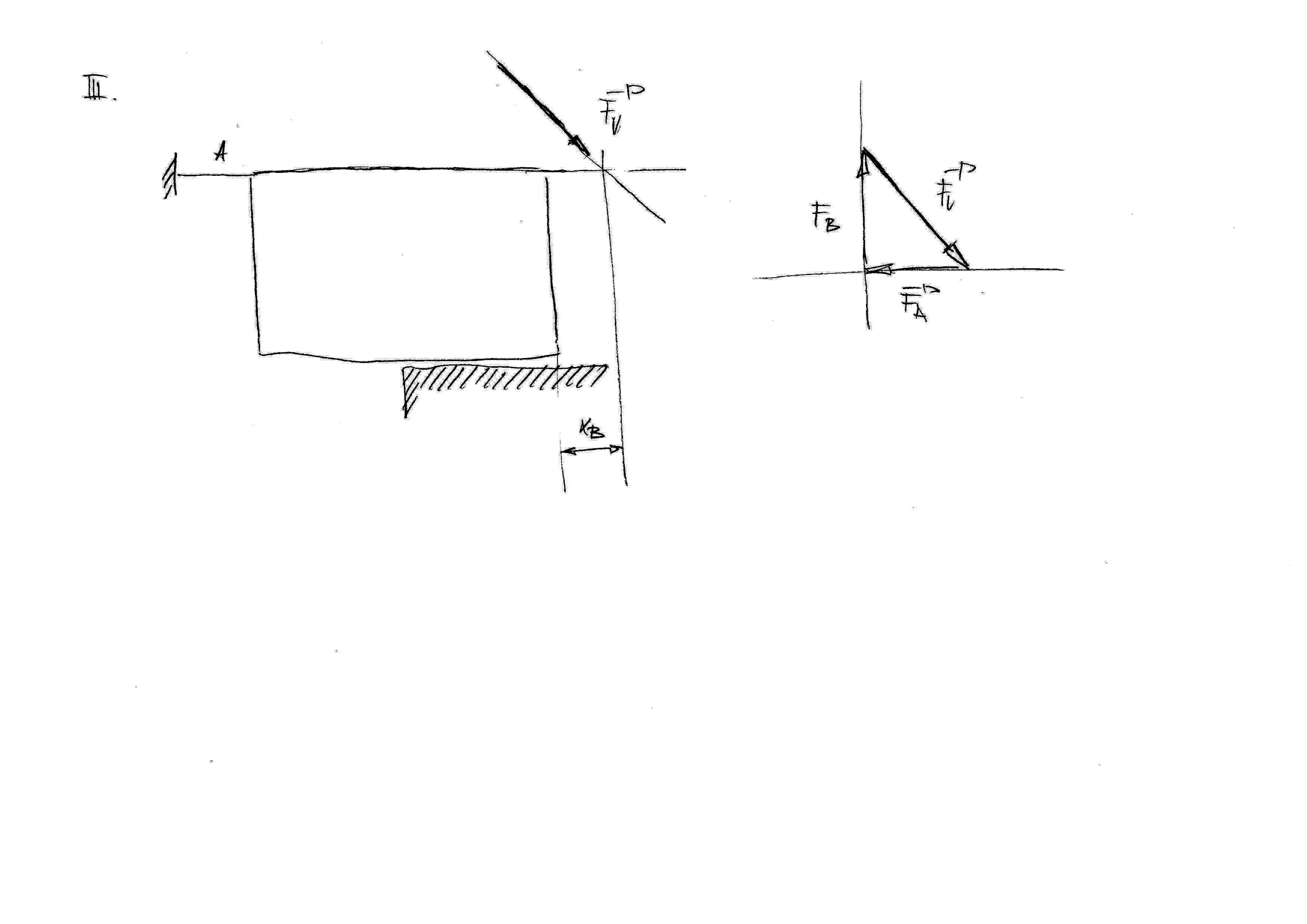
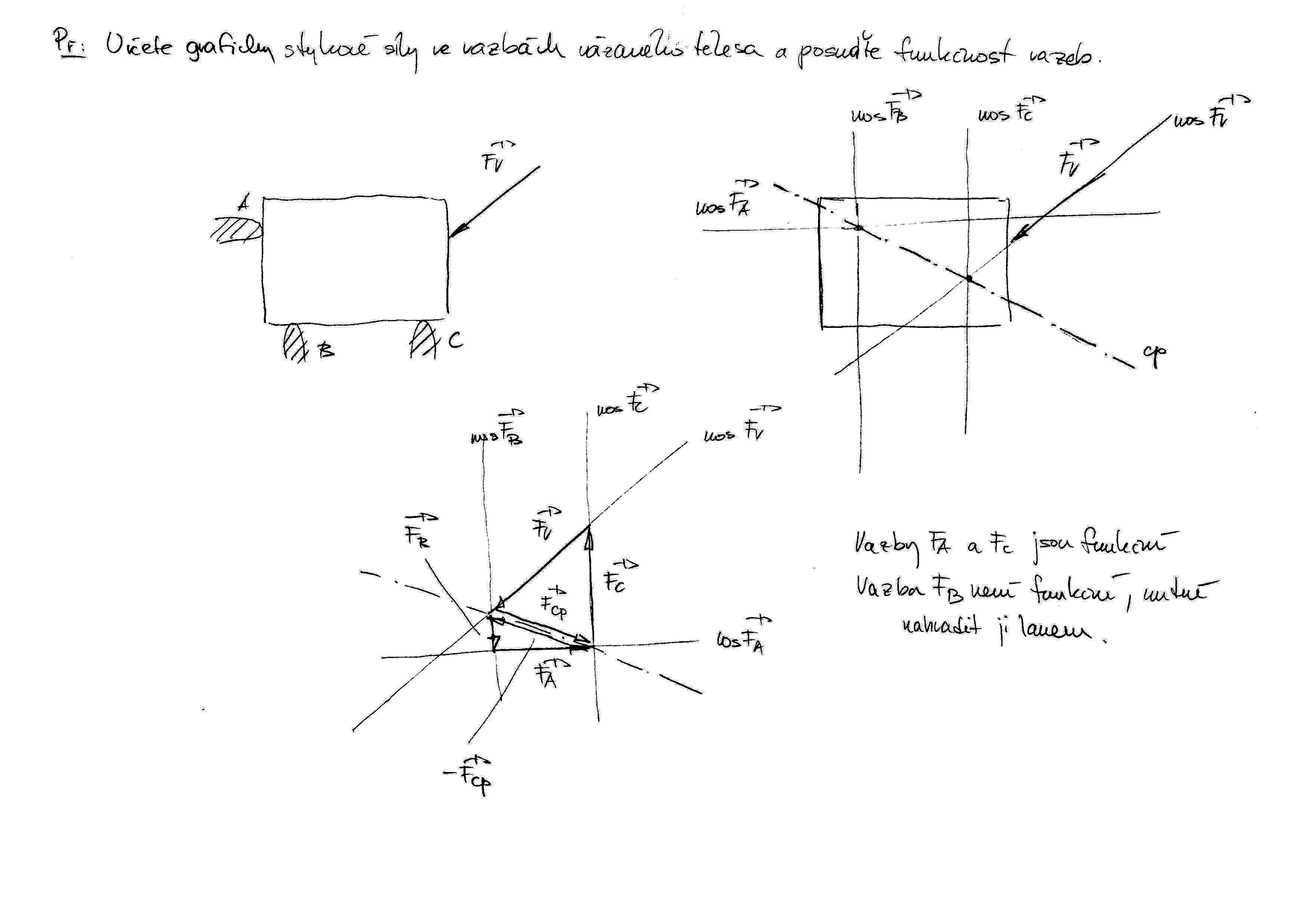
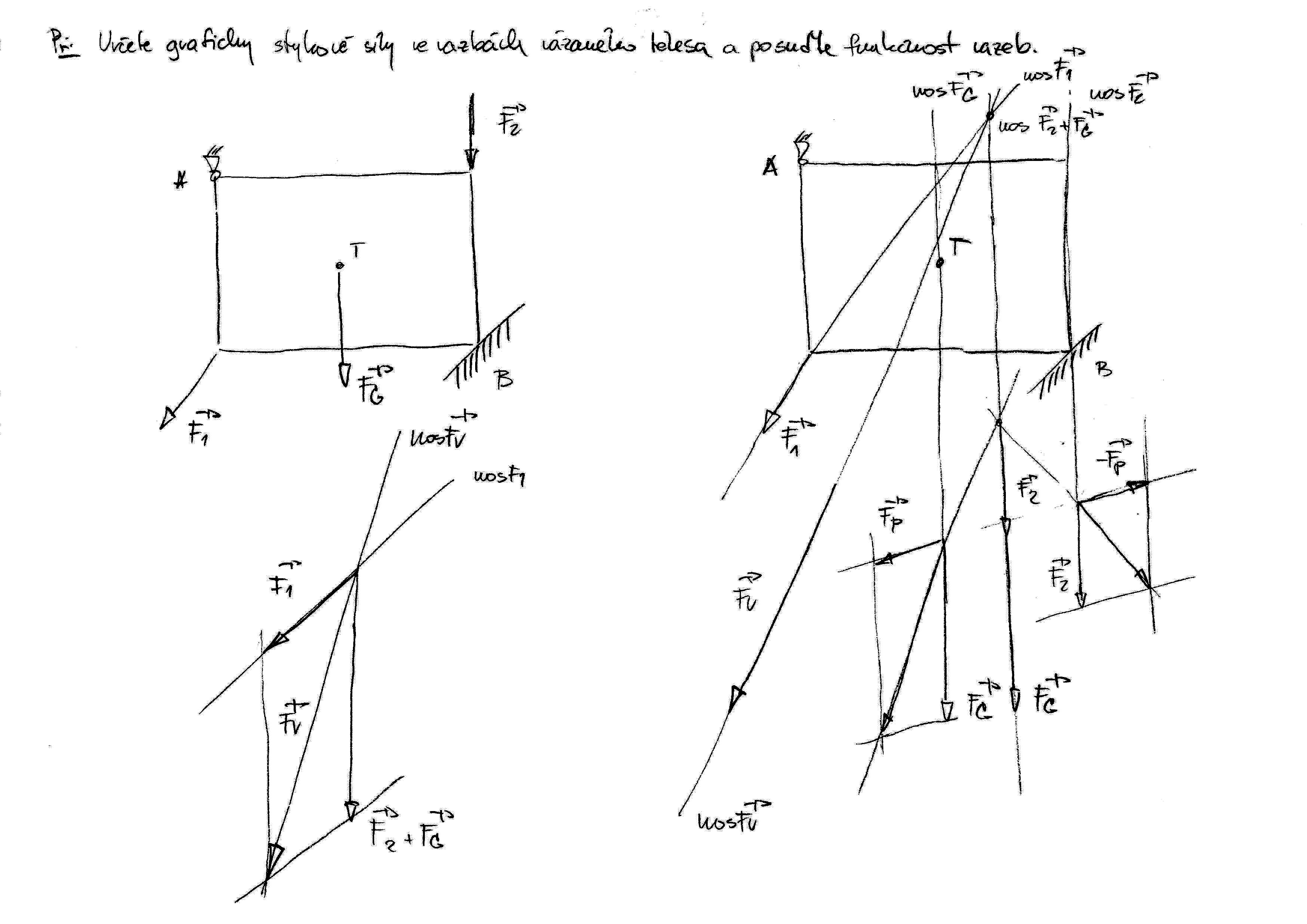
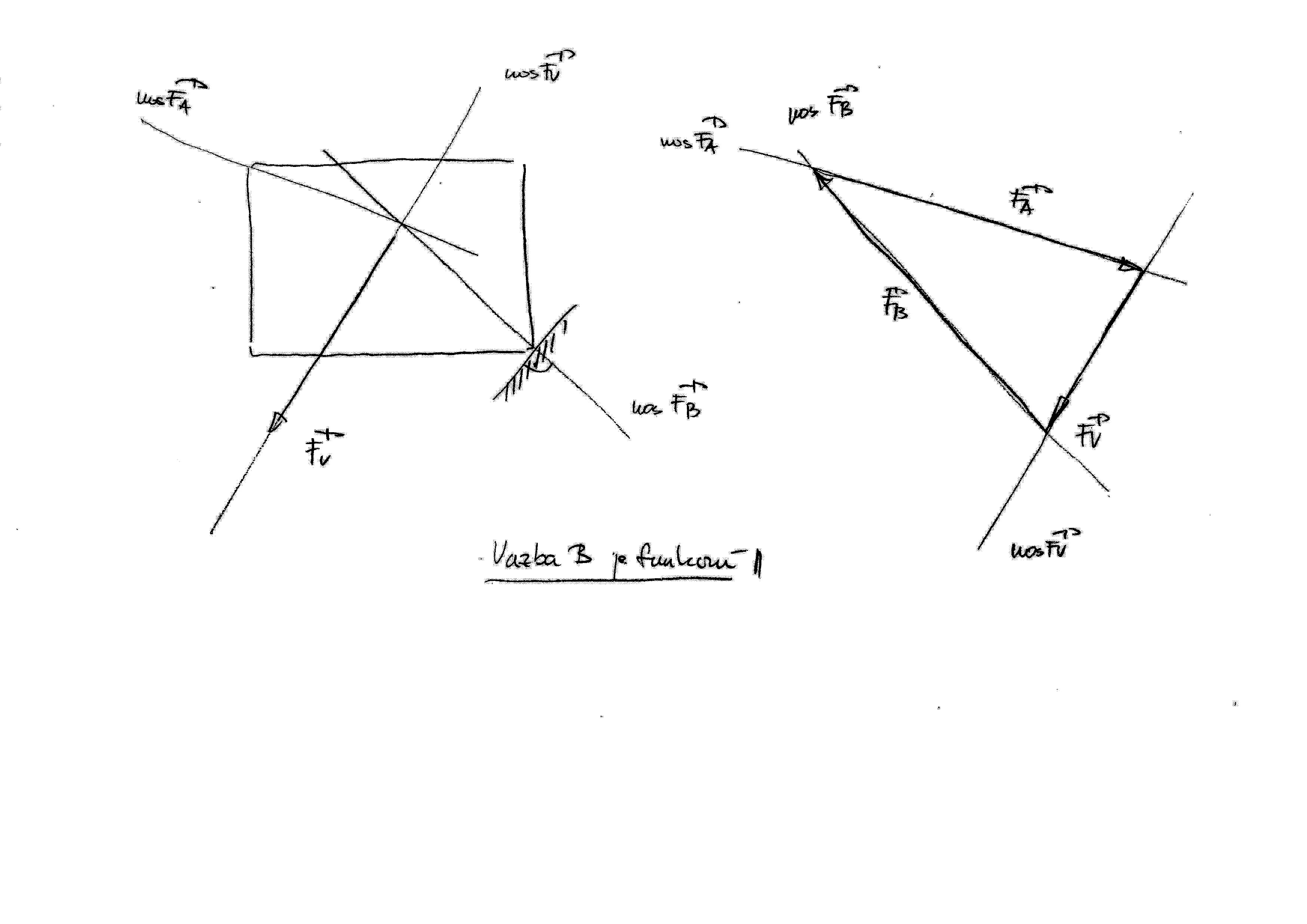
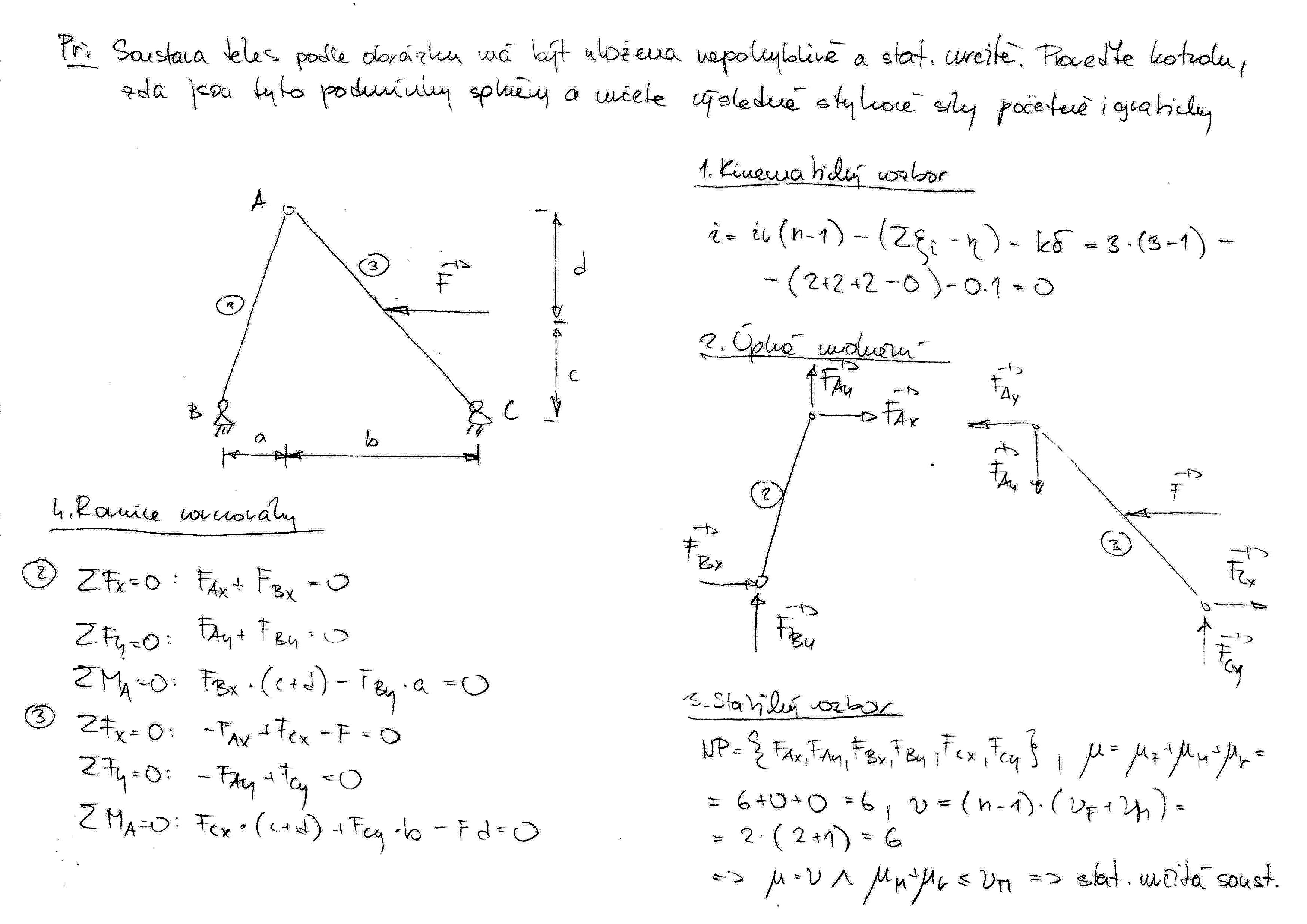
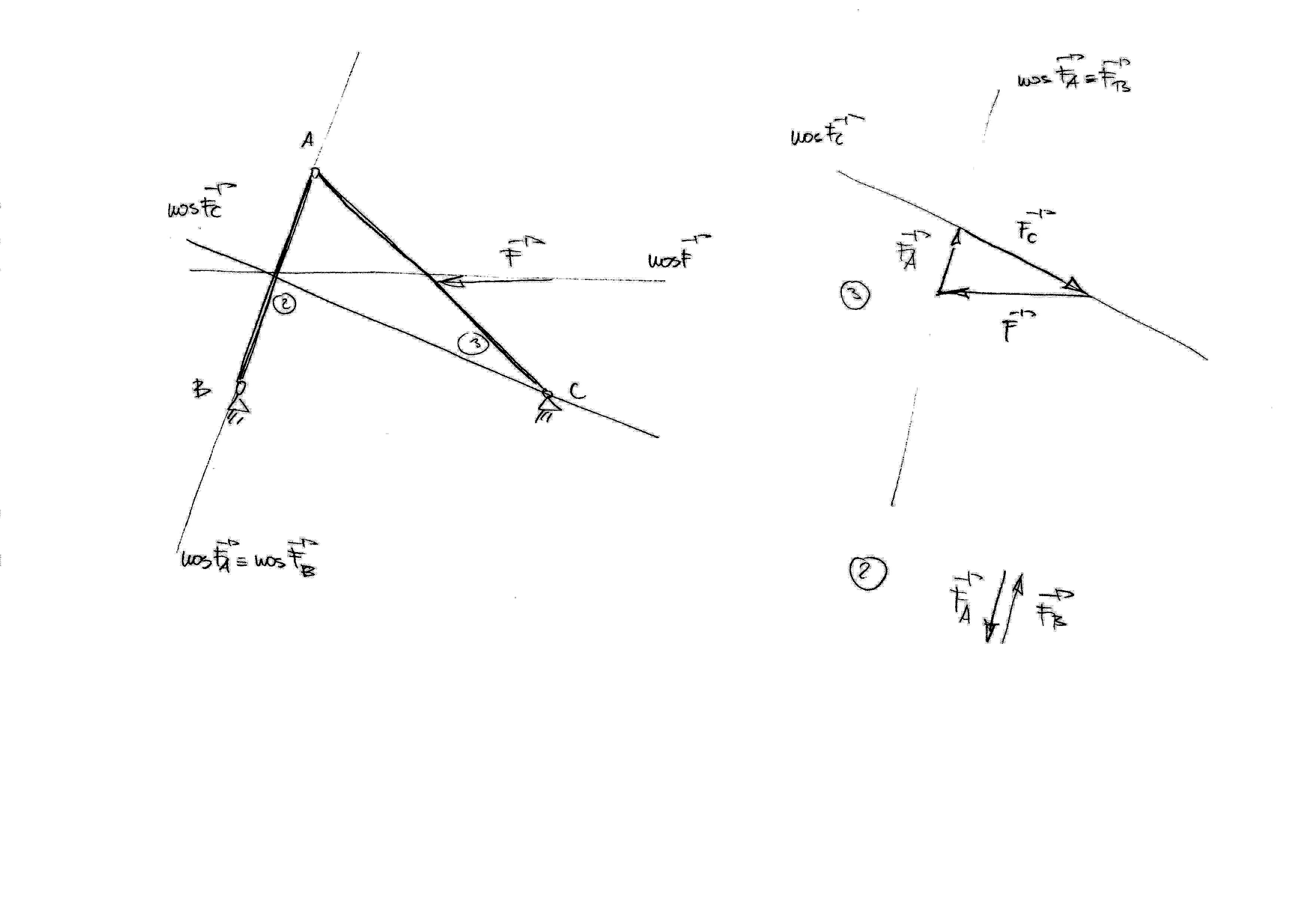
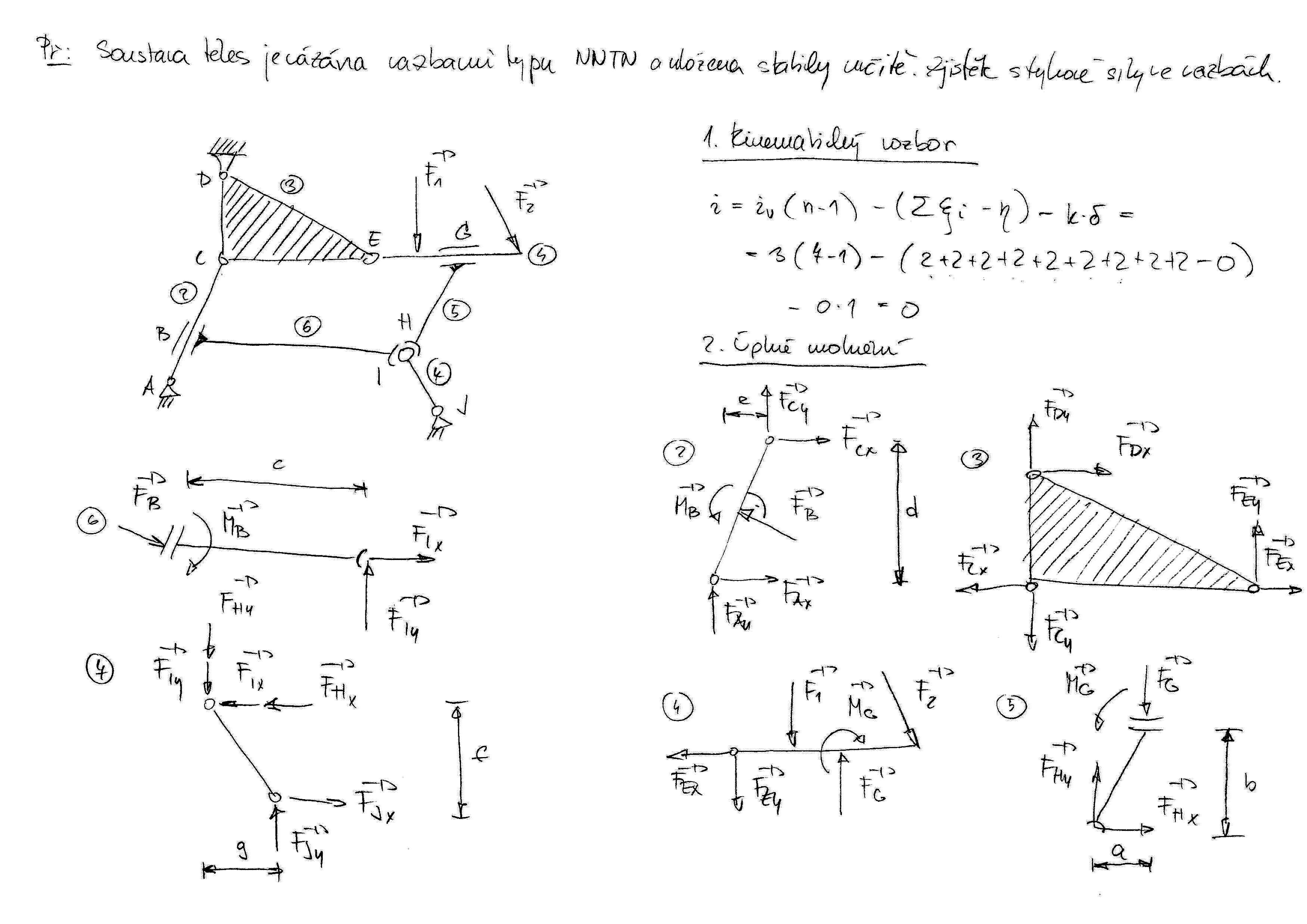
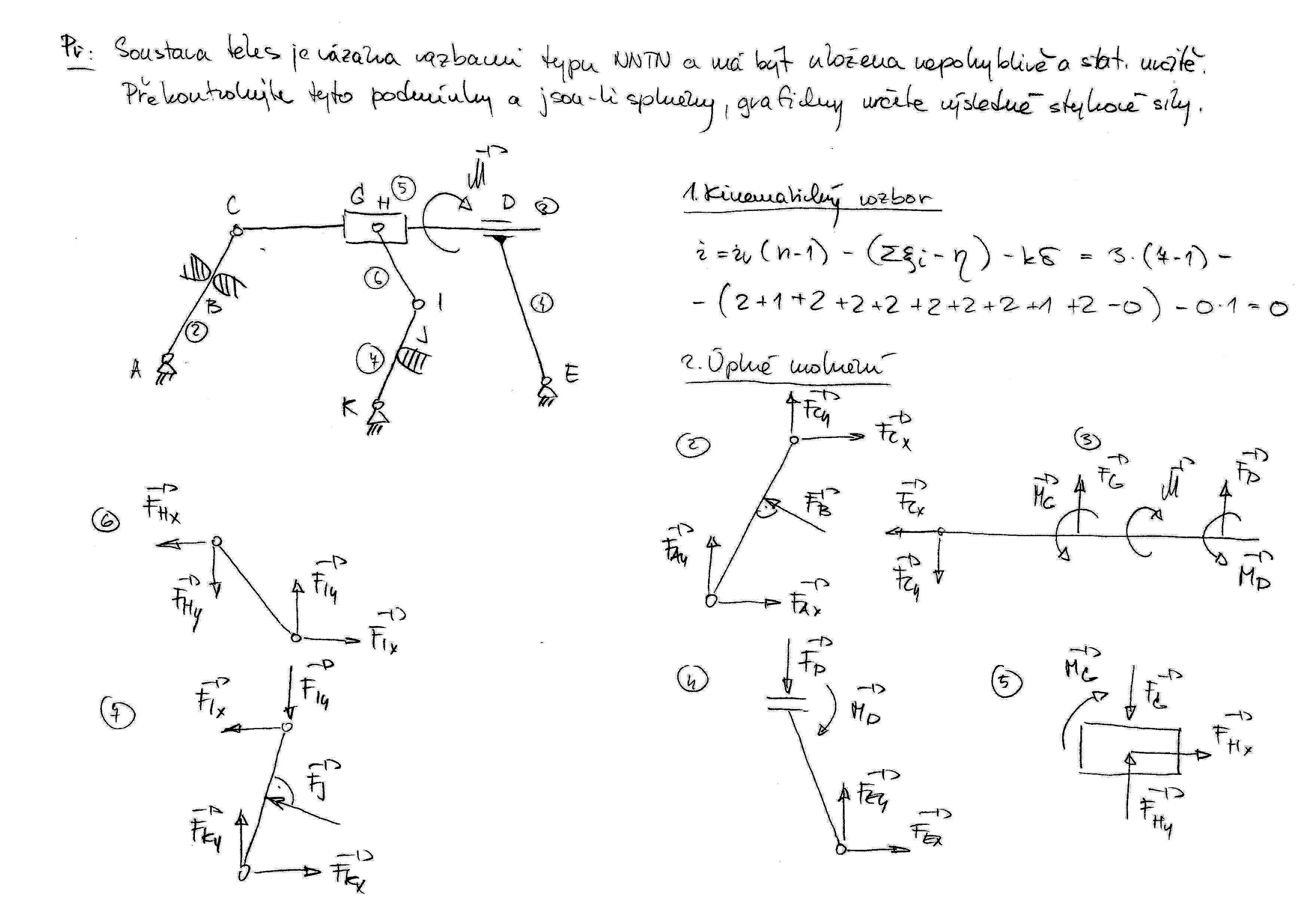
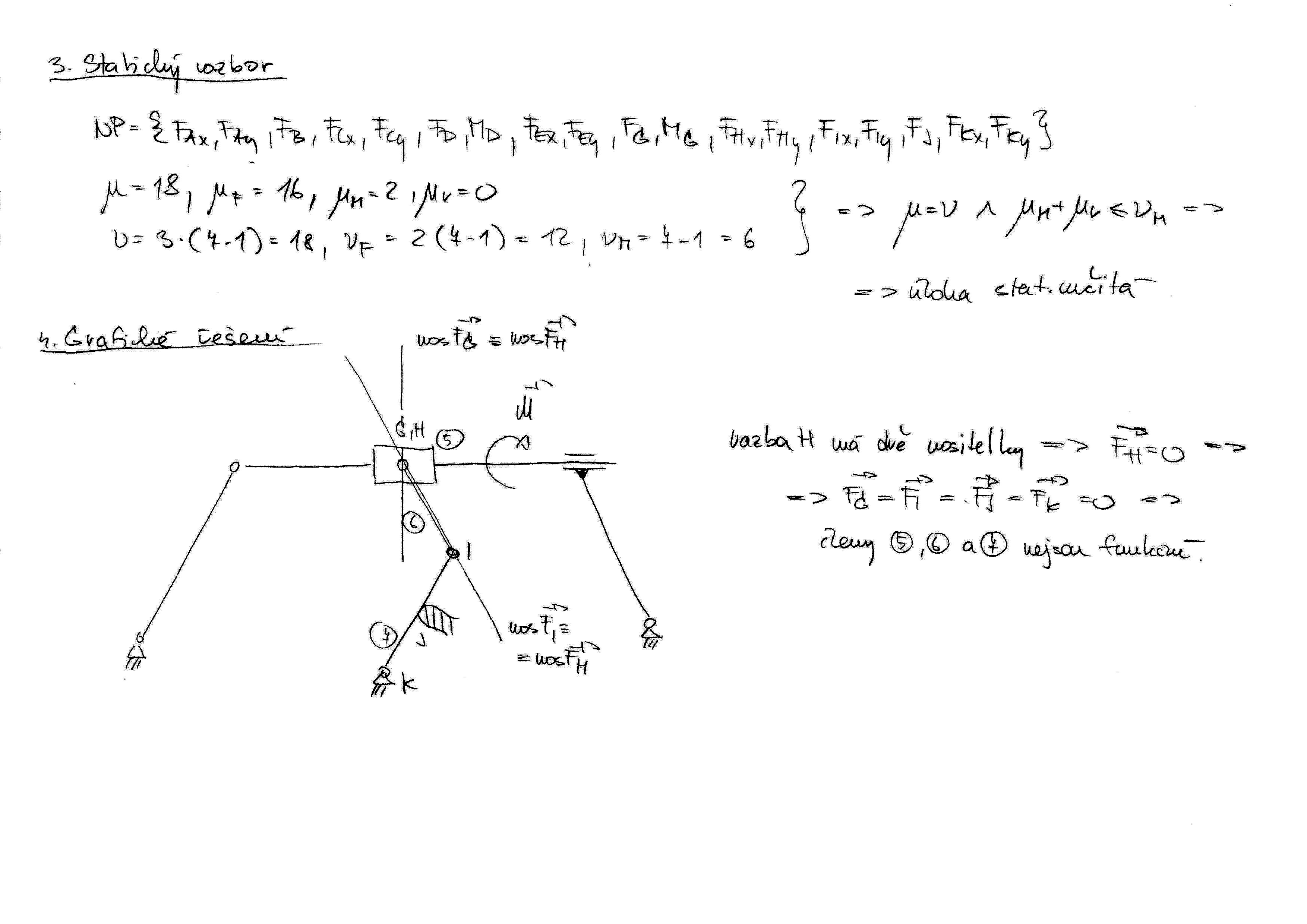
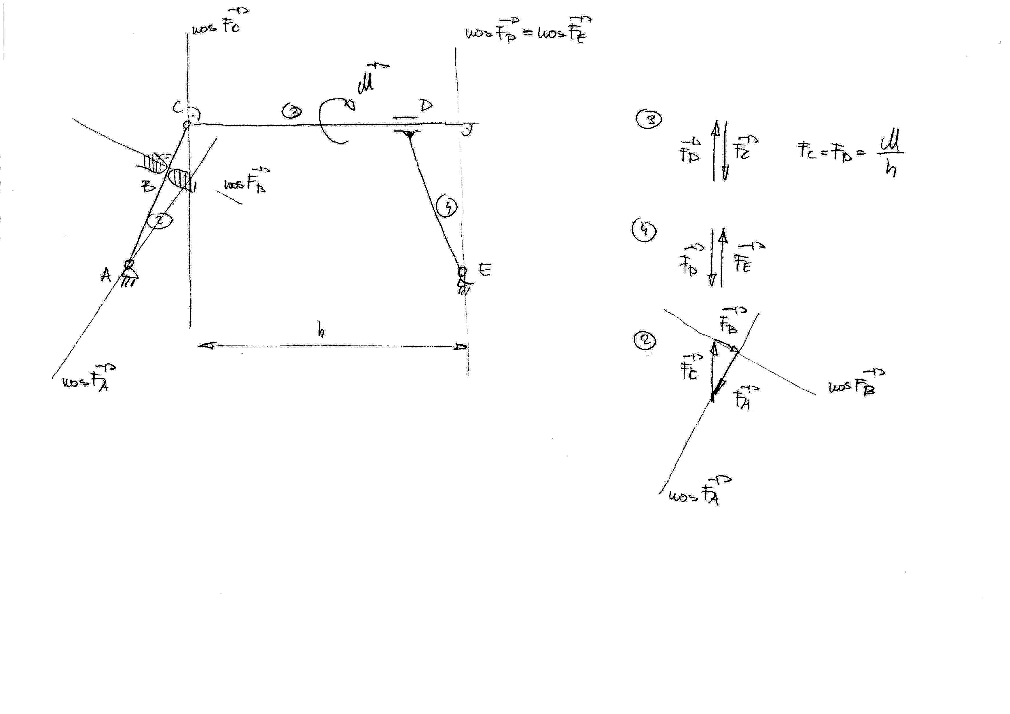
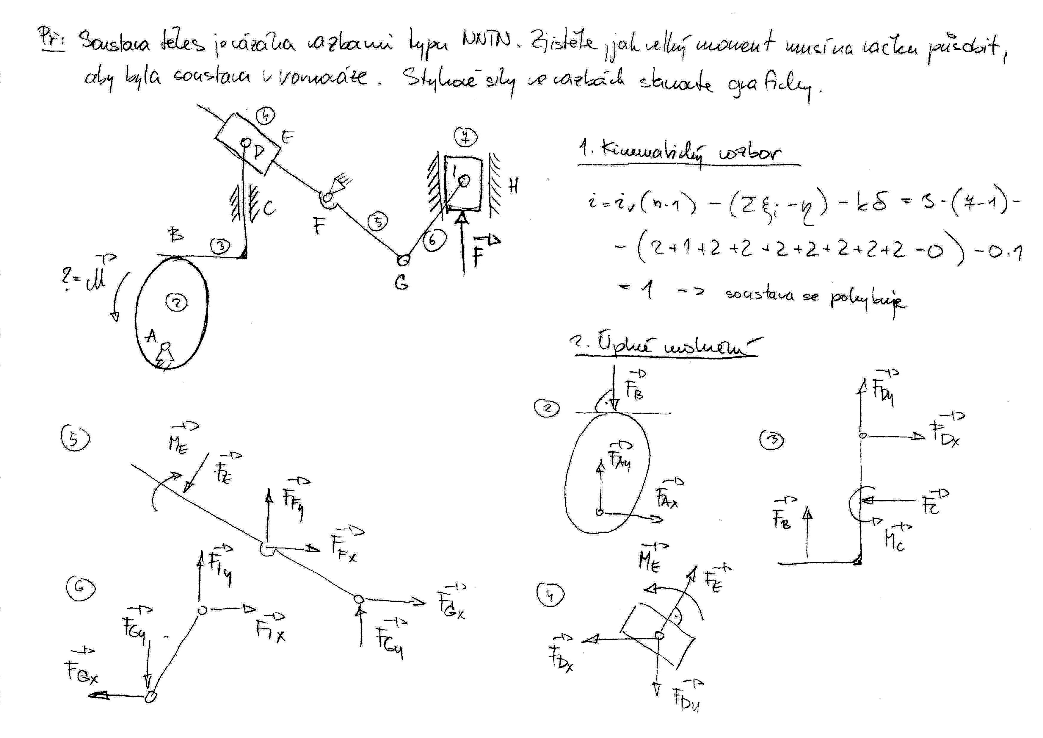
  • Cvičení 7: Vázané těleso, soustava těles.

    • Ručně řešený příklad Př.1 lze stáhnout zde a zde.

    • Ručně řešený příklad Př.2 lze stáhnout zde.

    • Ručně řešený příklad Př.3 lze stáhnout zde a zde.

    • Soustava těles, obrázek lze stáhnout zde.

  • Cvičení 8: Soustava těles.

    • Ručně řešený příklad Př.1 lze stáhnout zde, zde, zde, zde a zde.

    • Ručně řešený příklad Př.2 lze stáhnout zde, zde a zde.

    • Ručně řešený příklad Př.3 lze stáhnout zde a zde.

    • Soustava těles, obrázek lze stáhnout zde.

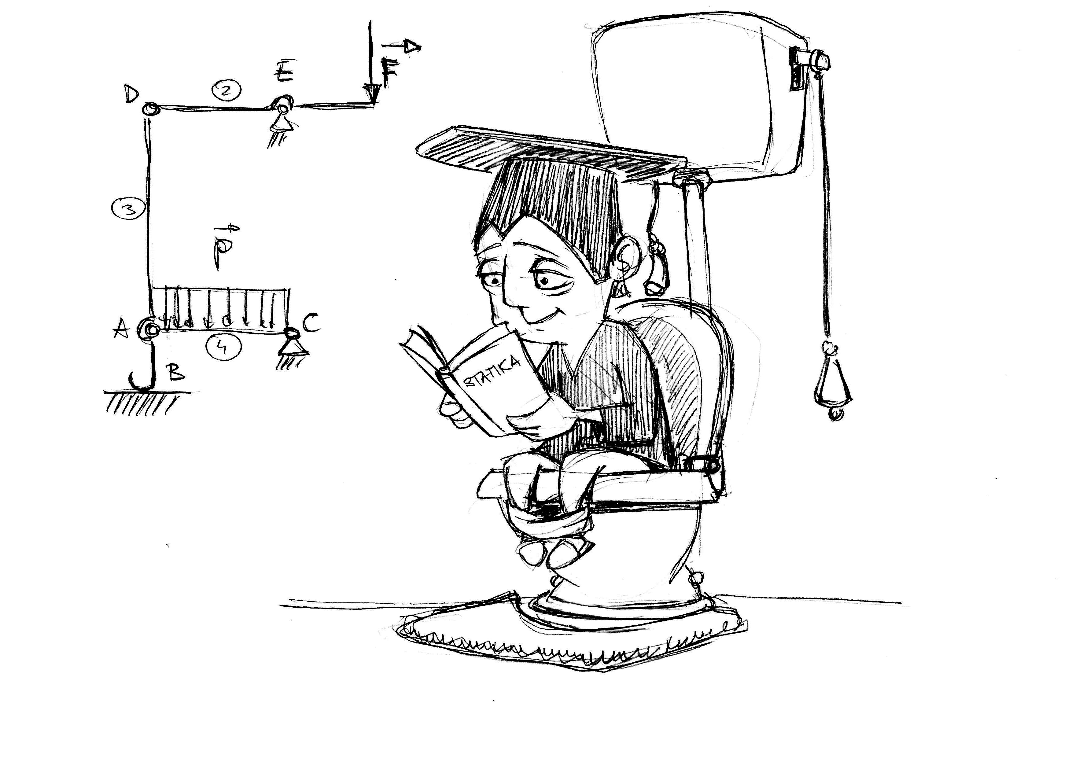
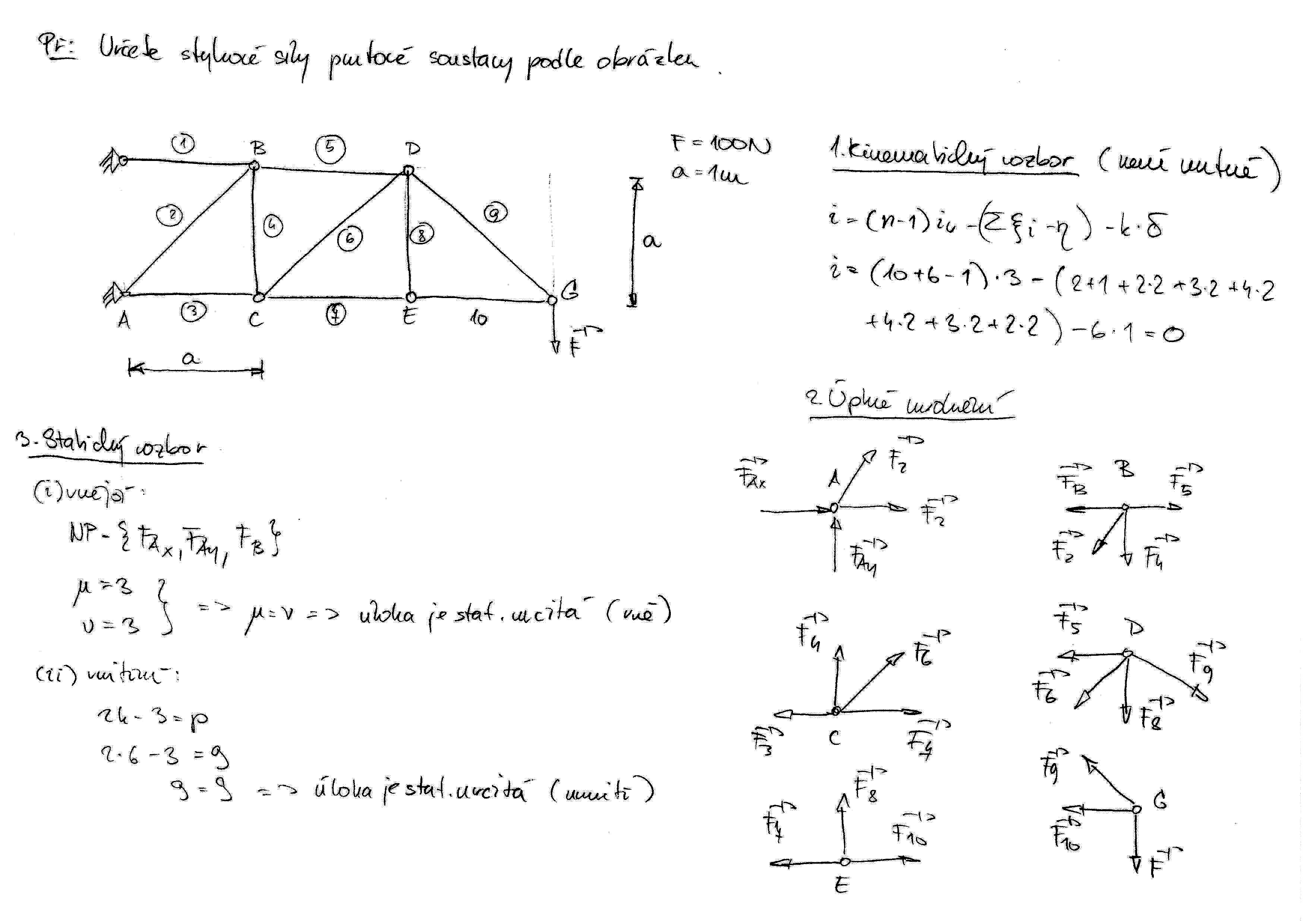
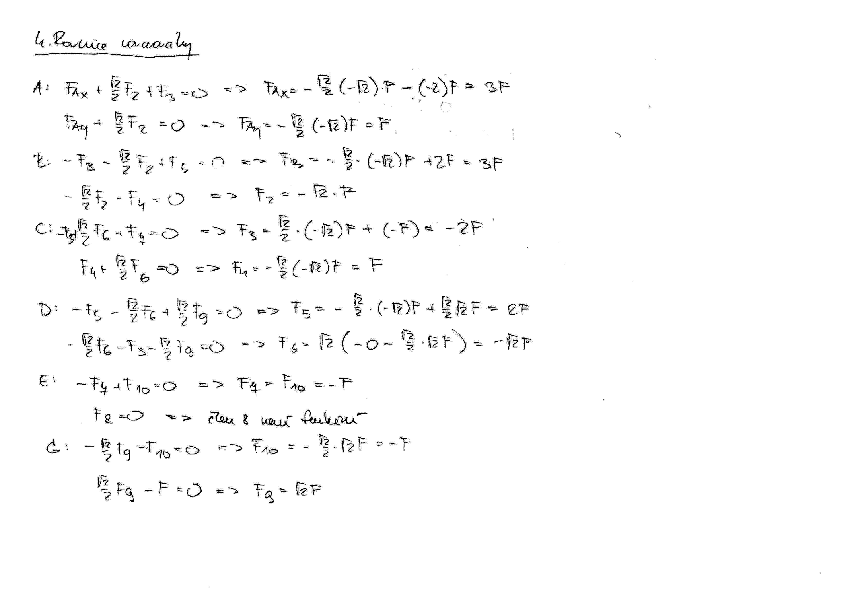
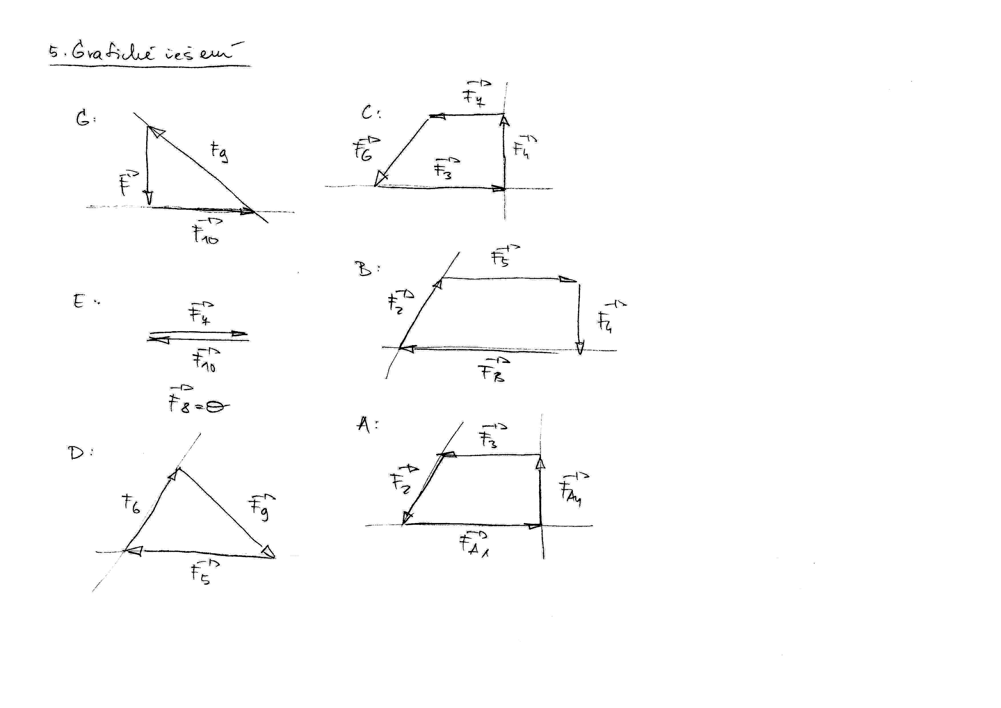
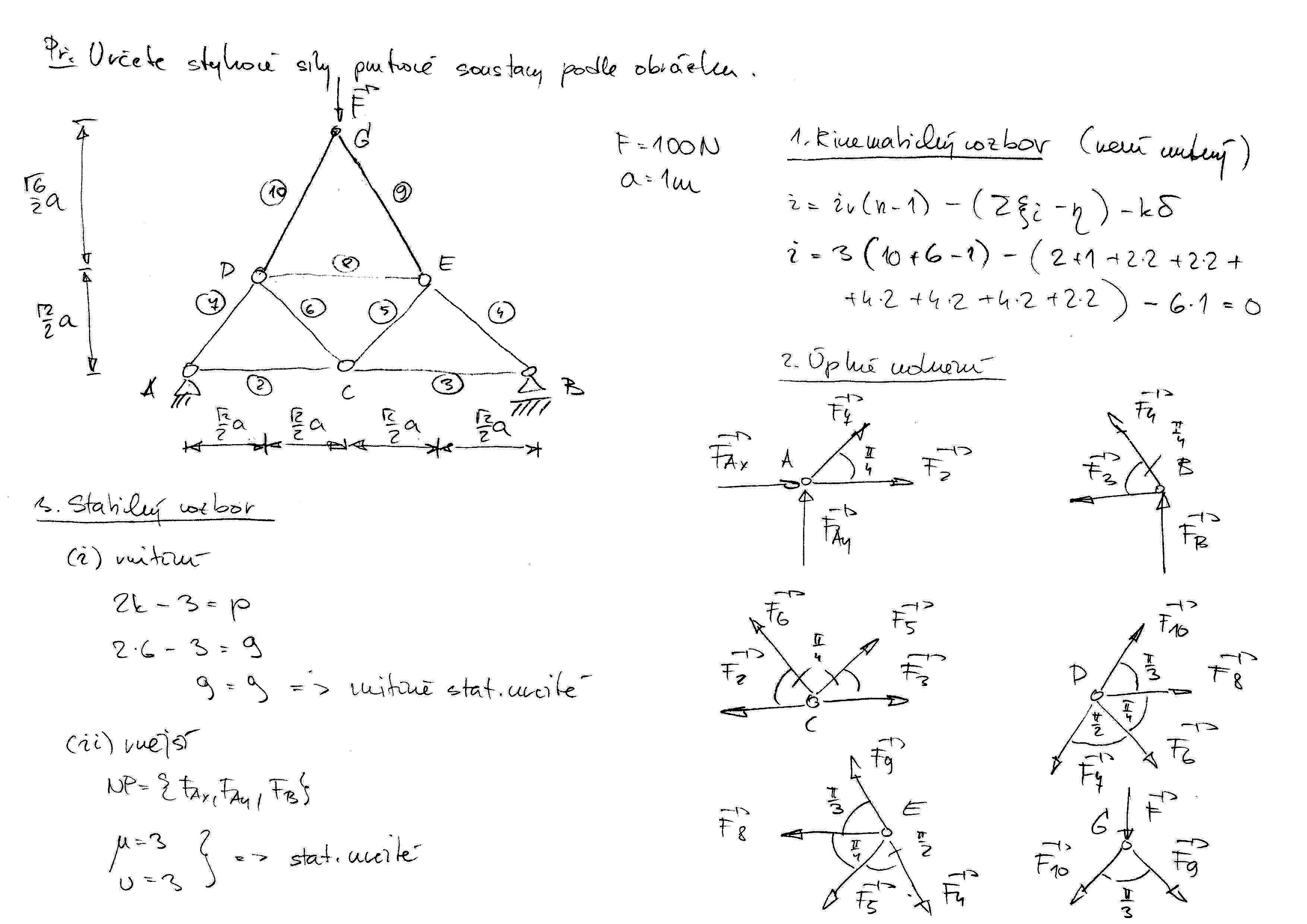
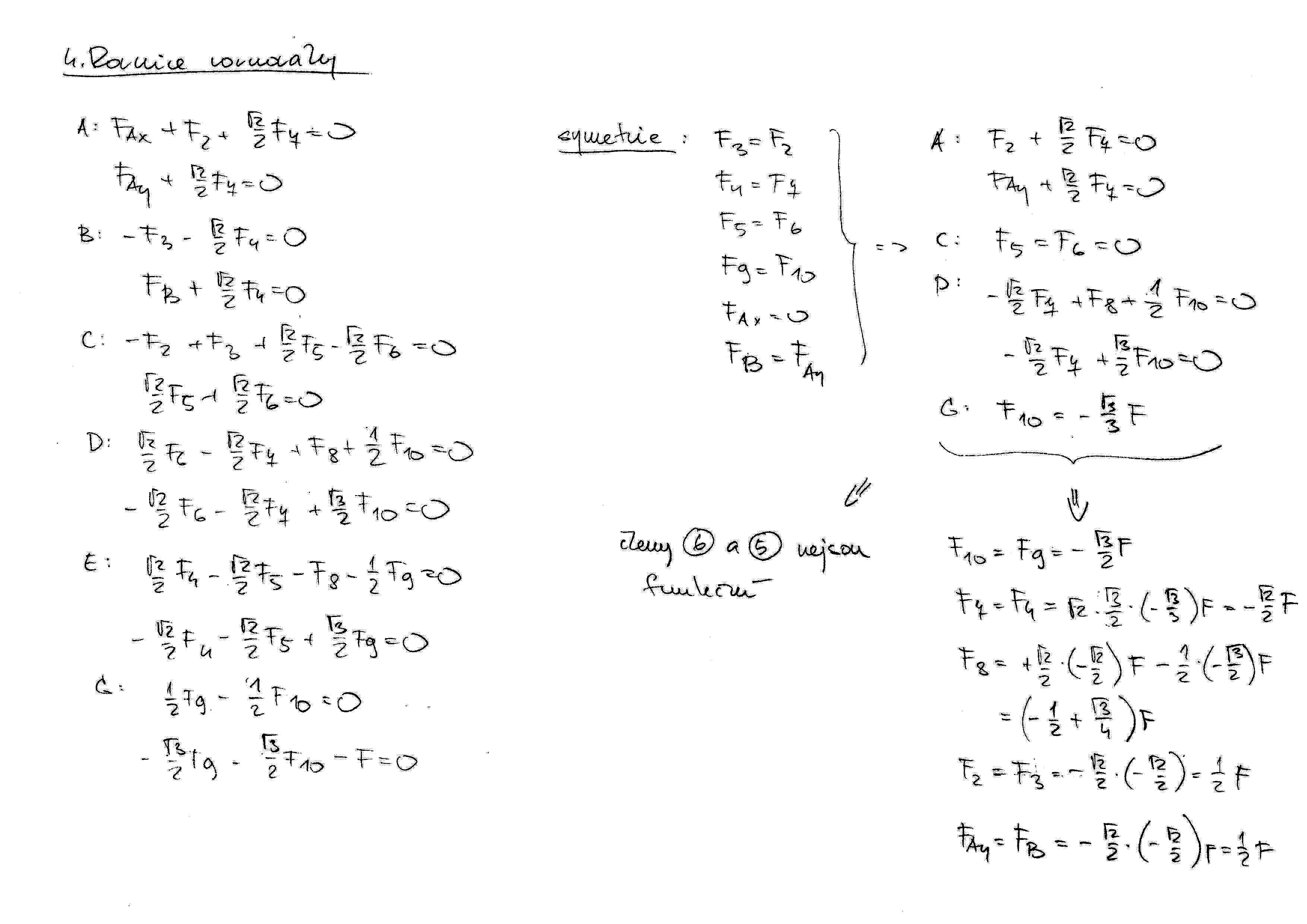
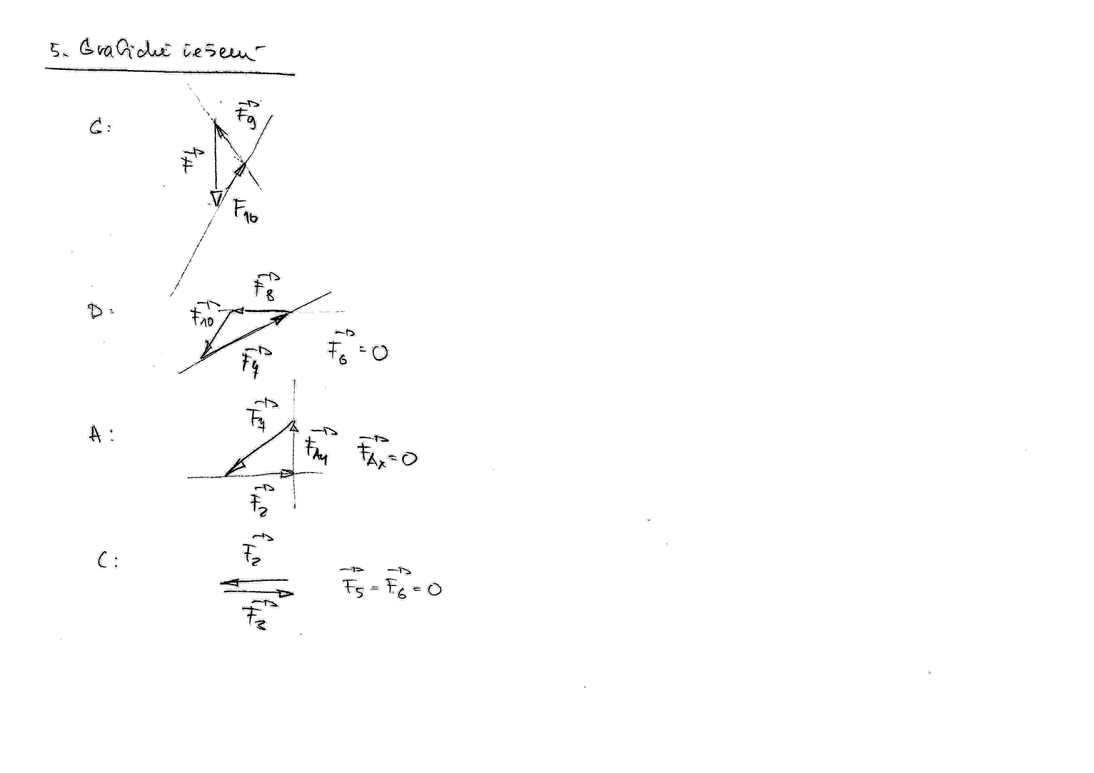
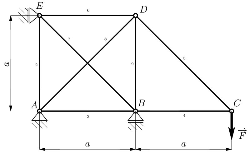
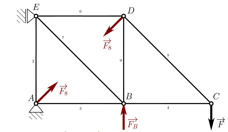
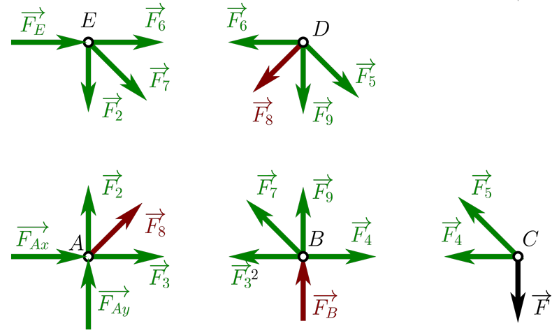
  • Cvičení 9: Prutová soustava

    • Ručně řešený příklad Př.1 lze stáhnout zde, zde a zde.

    • Ručně řešený příklad Př.2 lze stáhnout zde, zde a zde.

    • Centrální silová soustava, obrázek lze stáhnout zde.

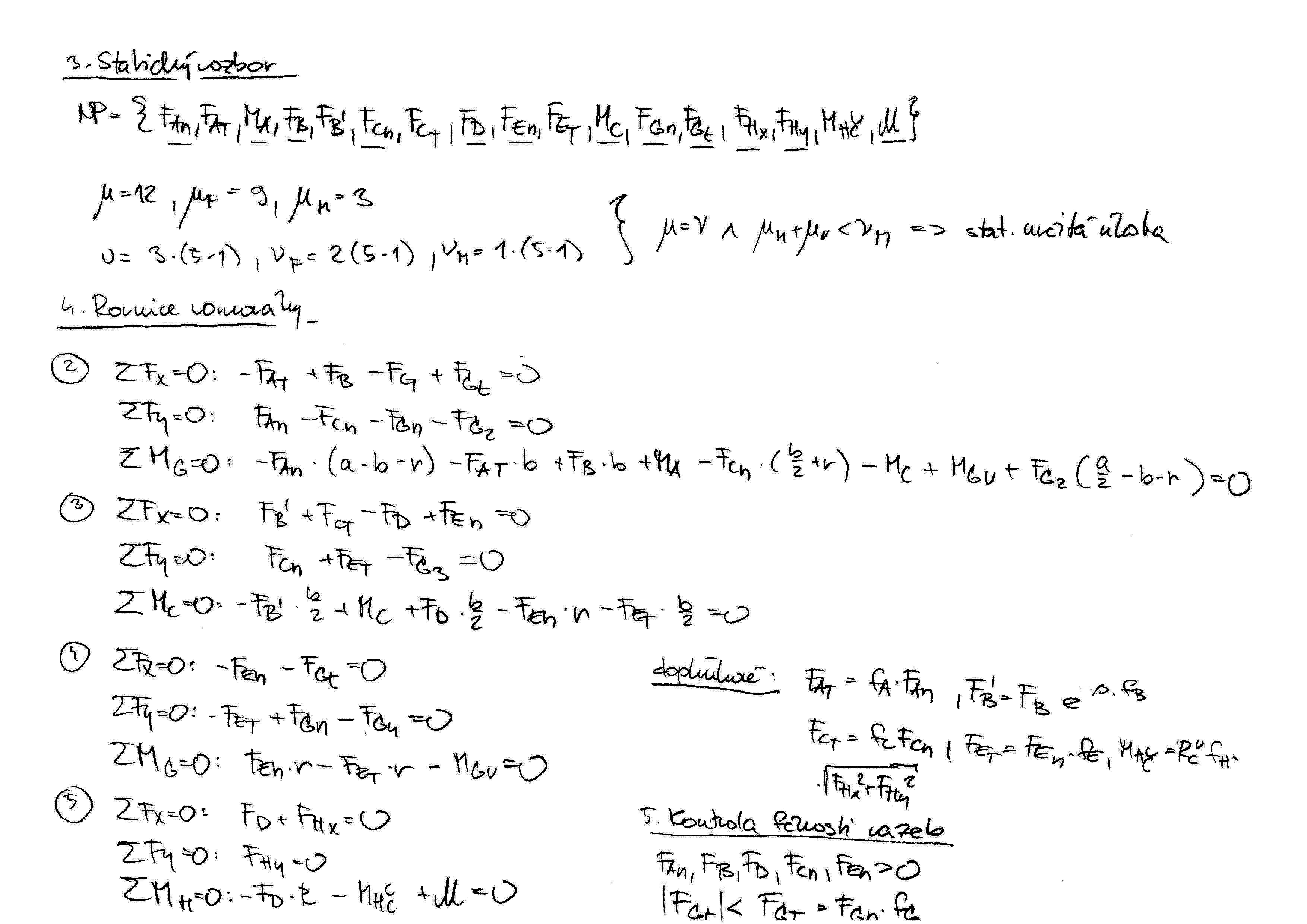
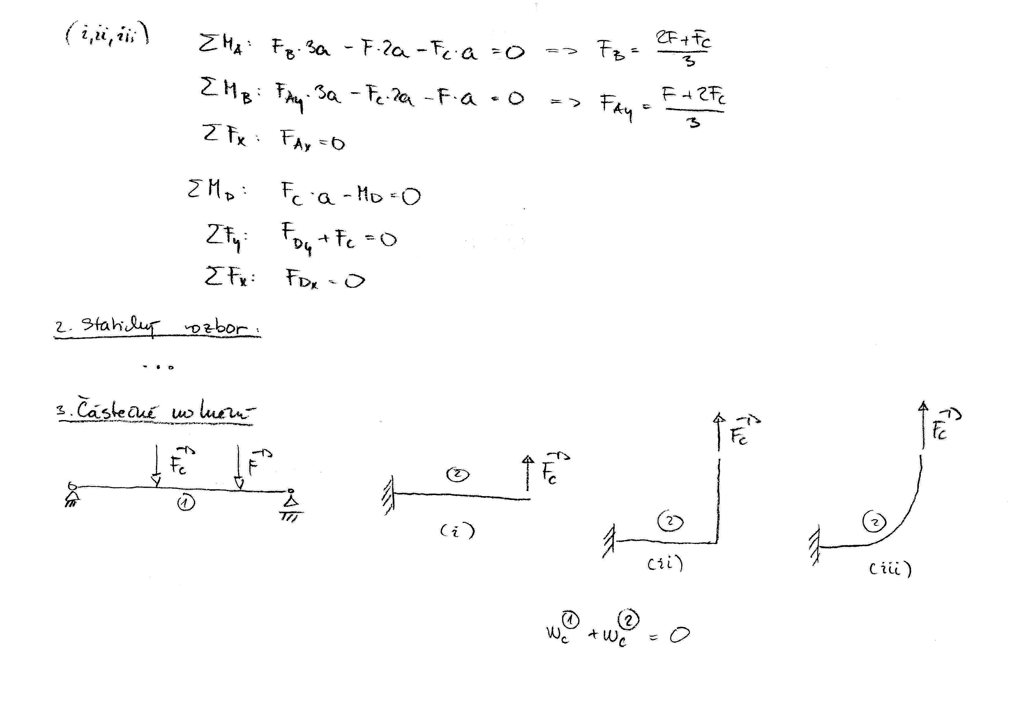
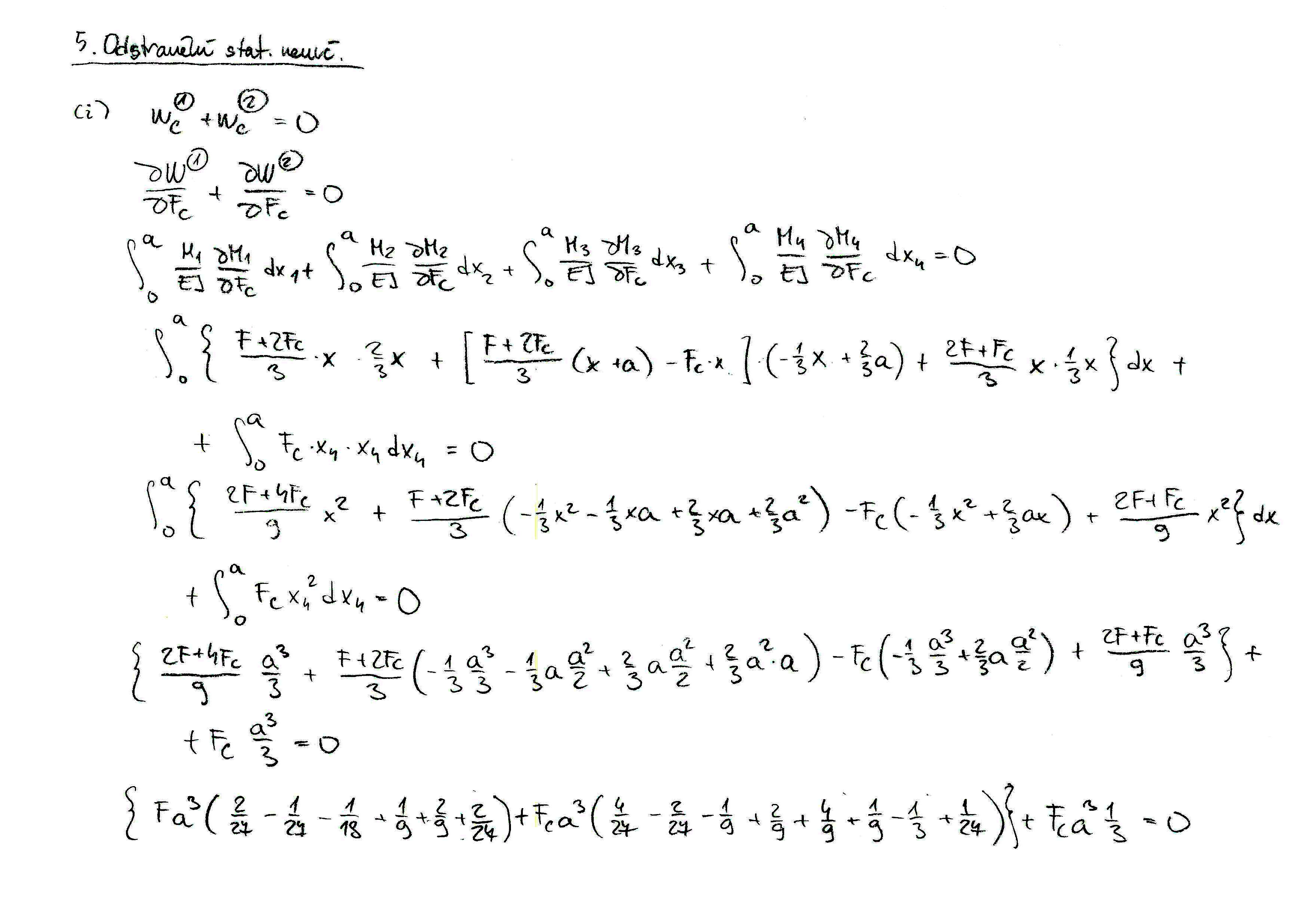
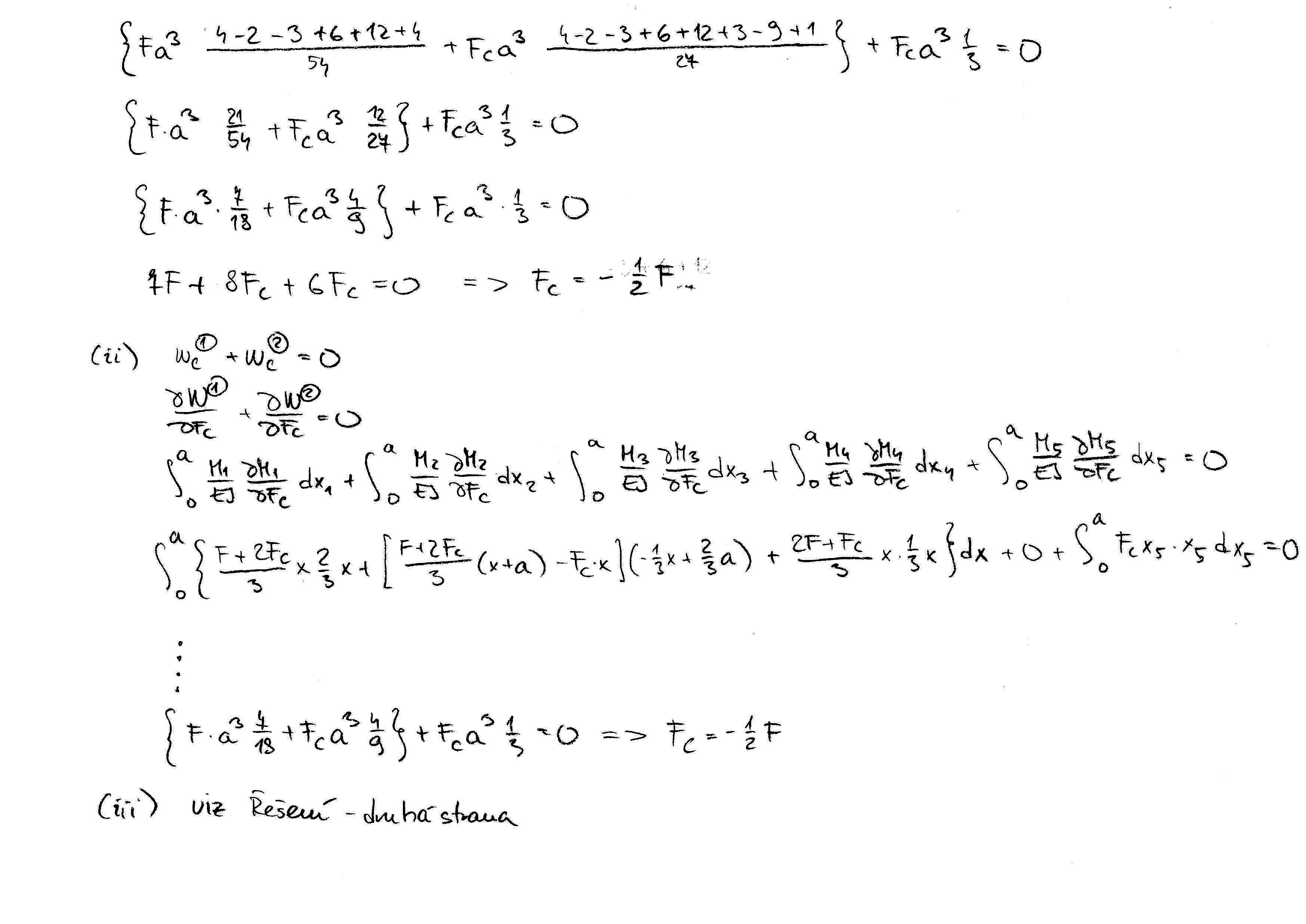
  • Cvičení 10: Pasívní účinky

    • Ručně řešený příklad Př.1 lze stáhnout zde a zde.

    • Ručně řešený příklad Př.2 lze stáhnout zde a zde.

  • Cvičení 11: Pasívní účinky

    • Ručně řešený příklad Př.1 lze stáhnout zde a zde.

    • Ručně řešený příklad Př.2 lze stáhnout zde a zde.

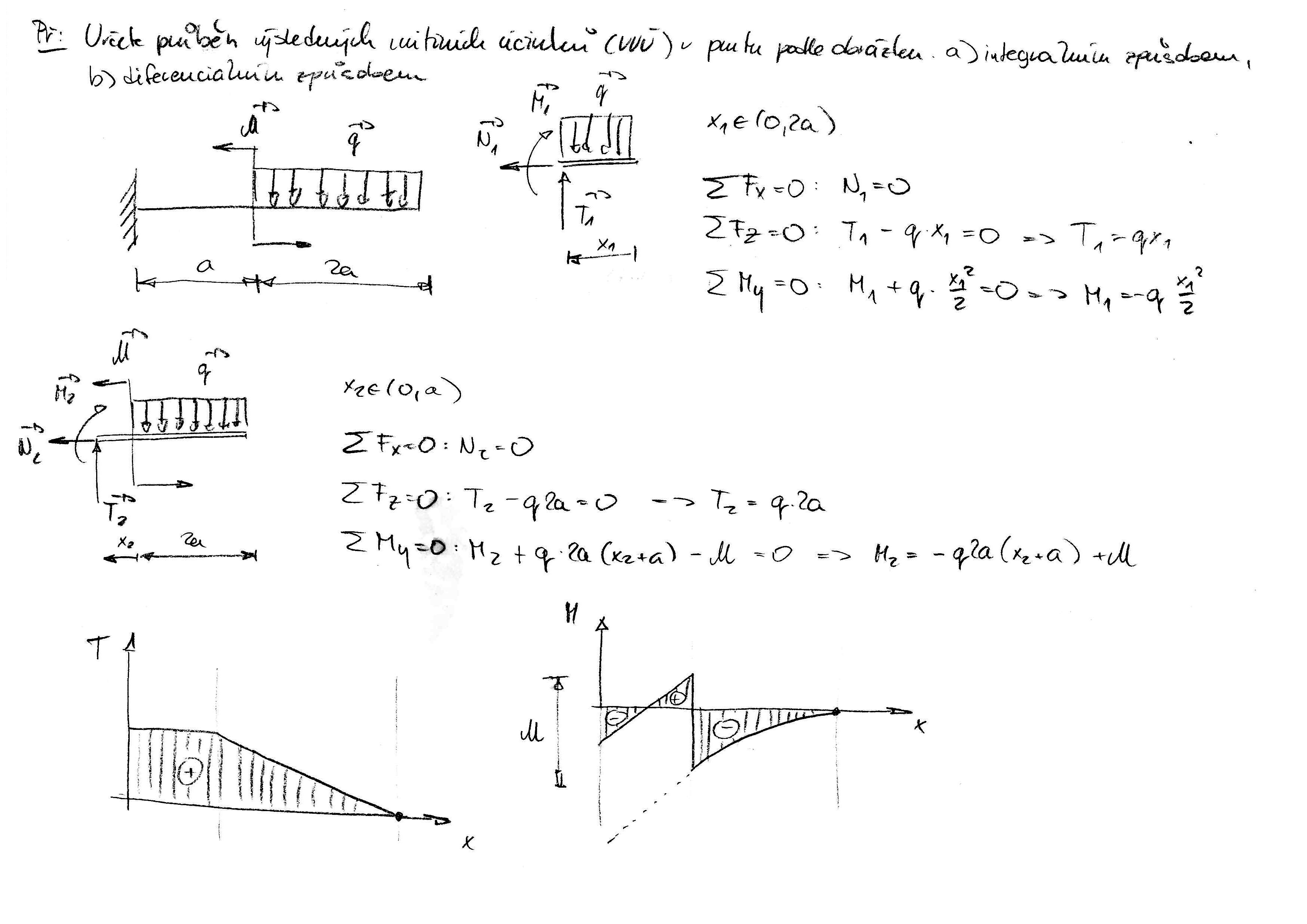
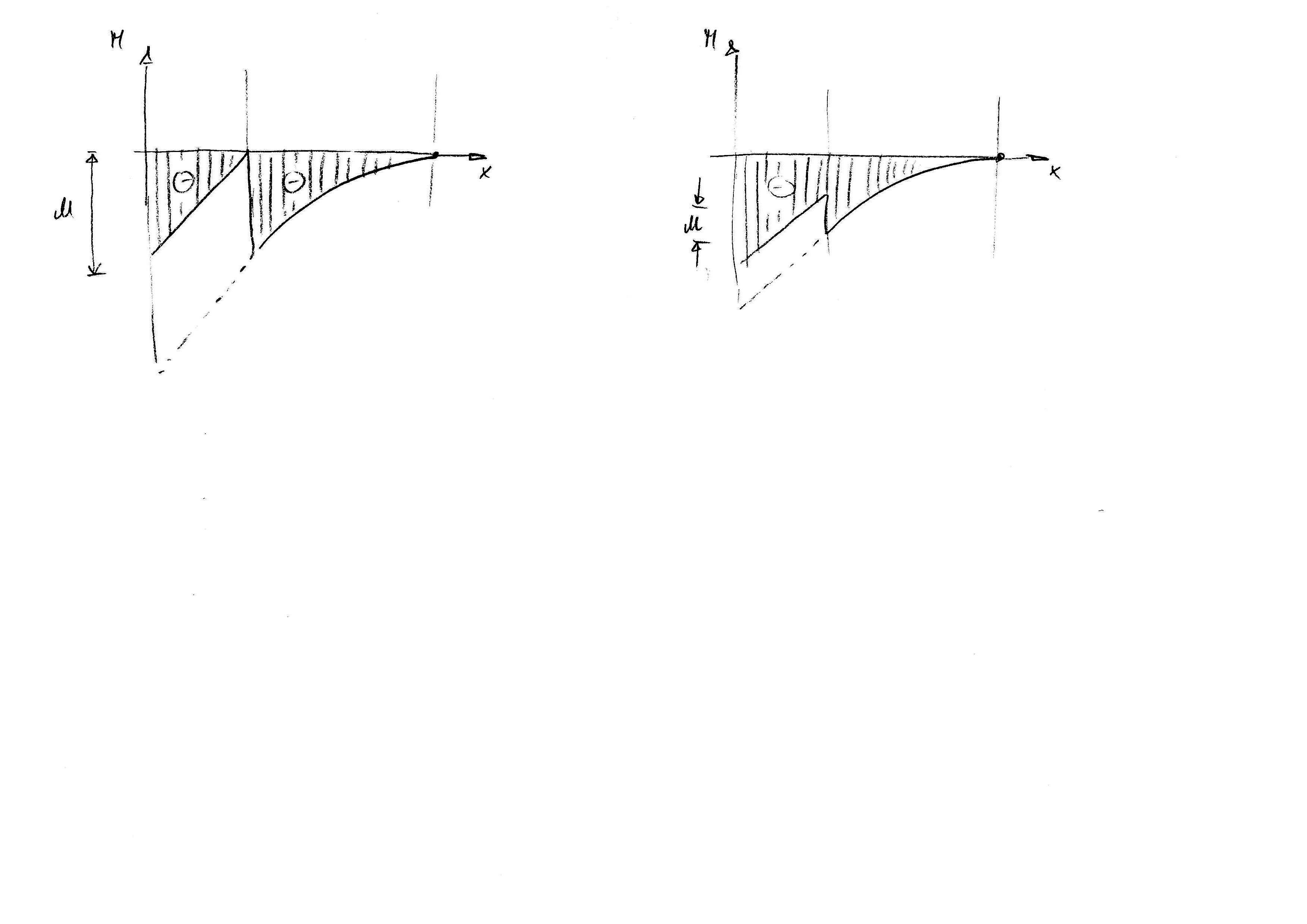
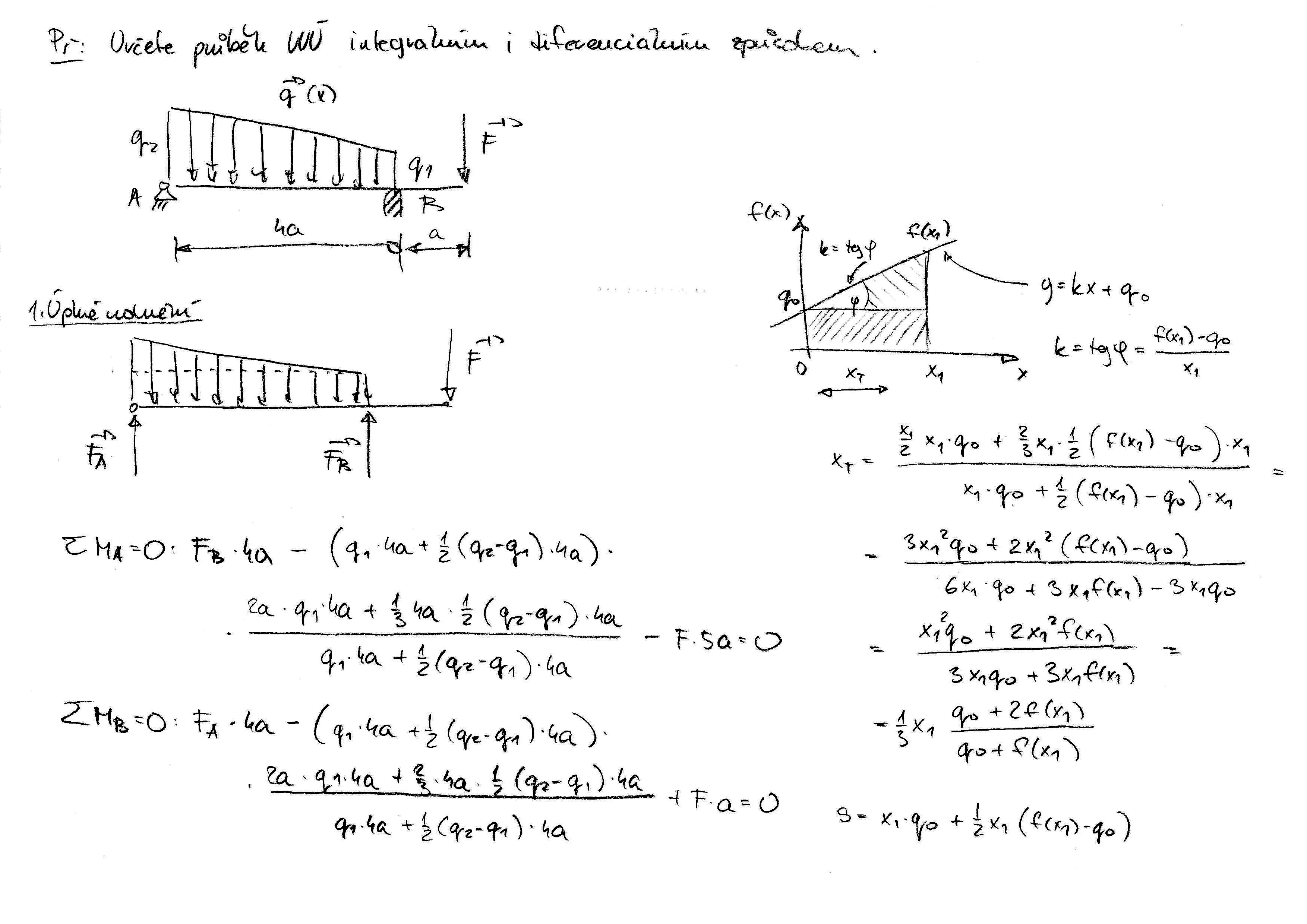
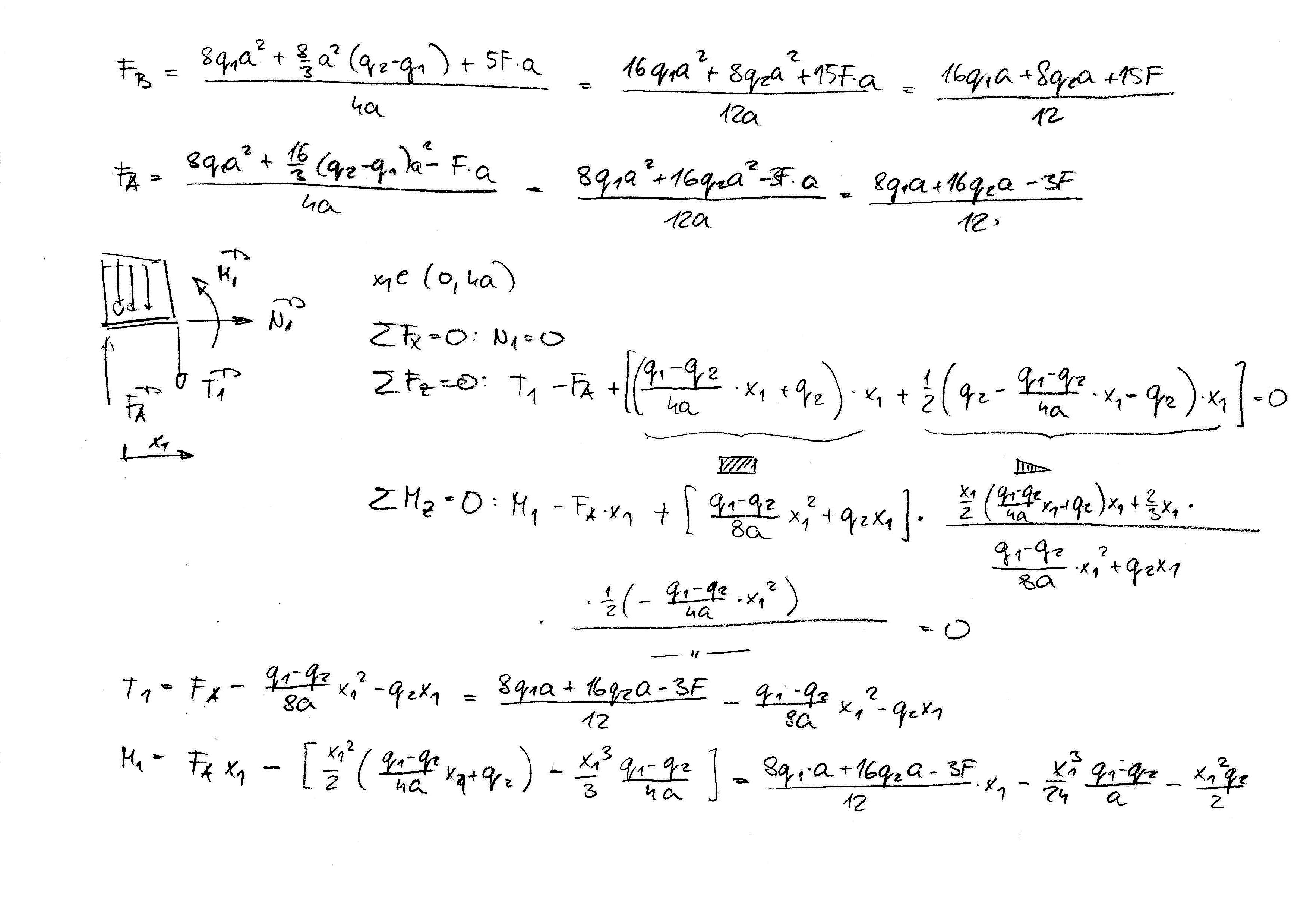
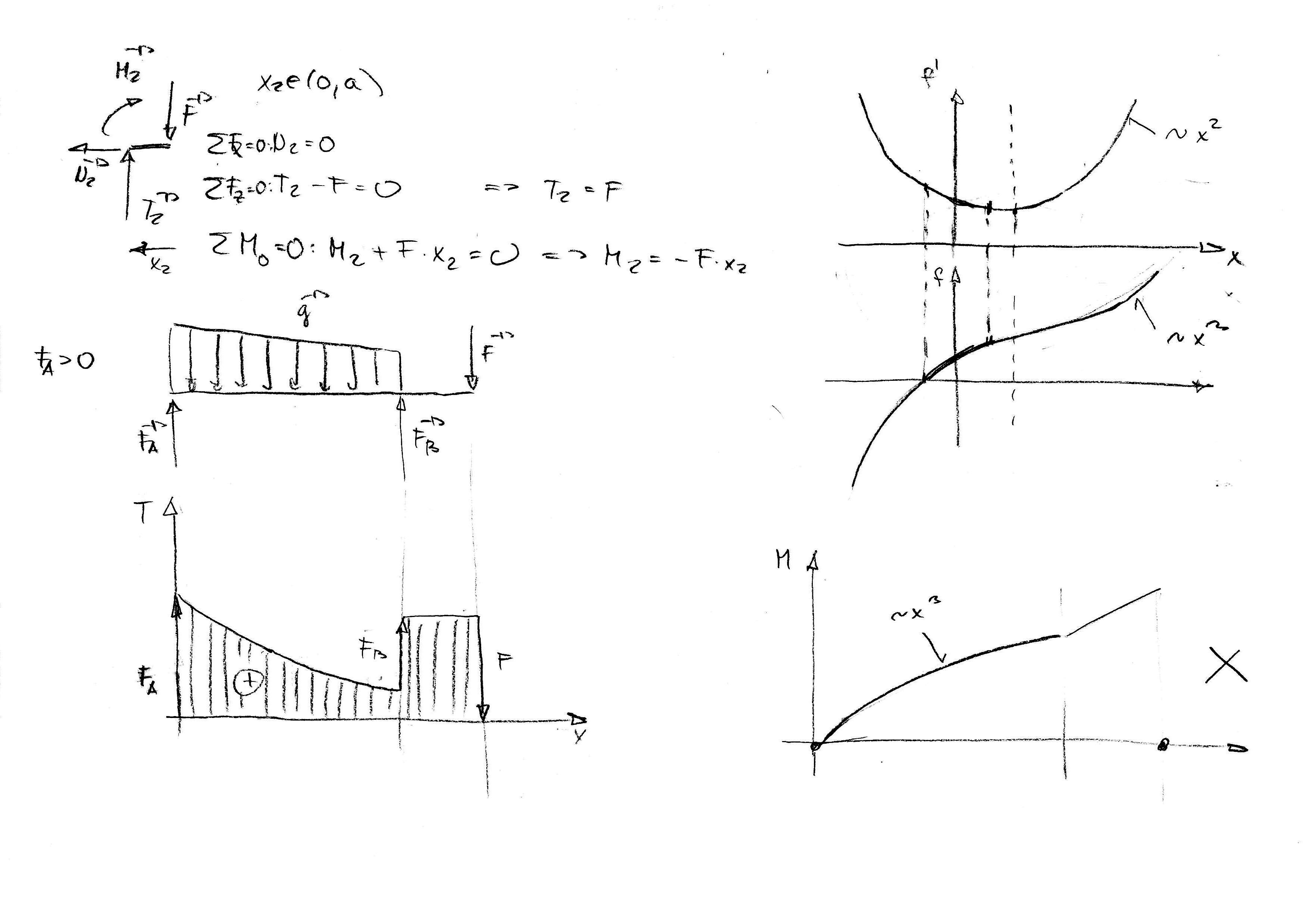
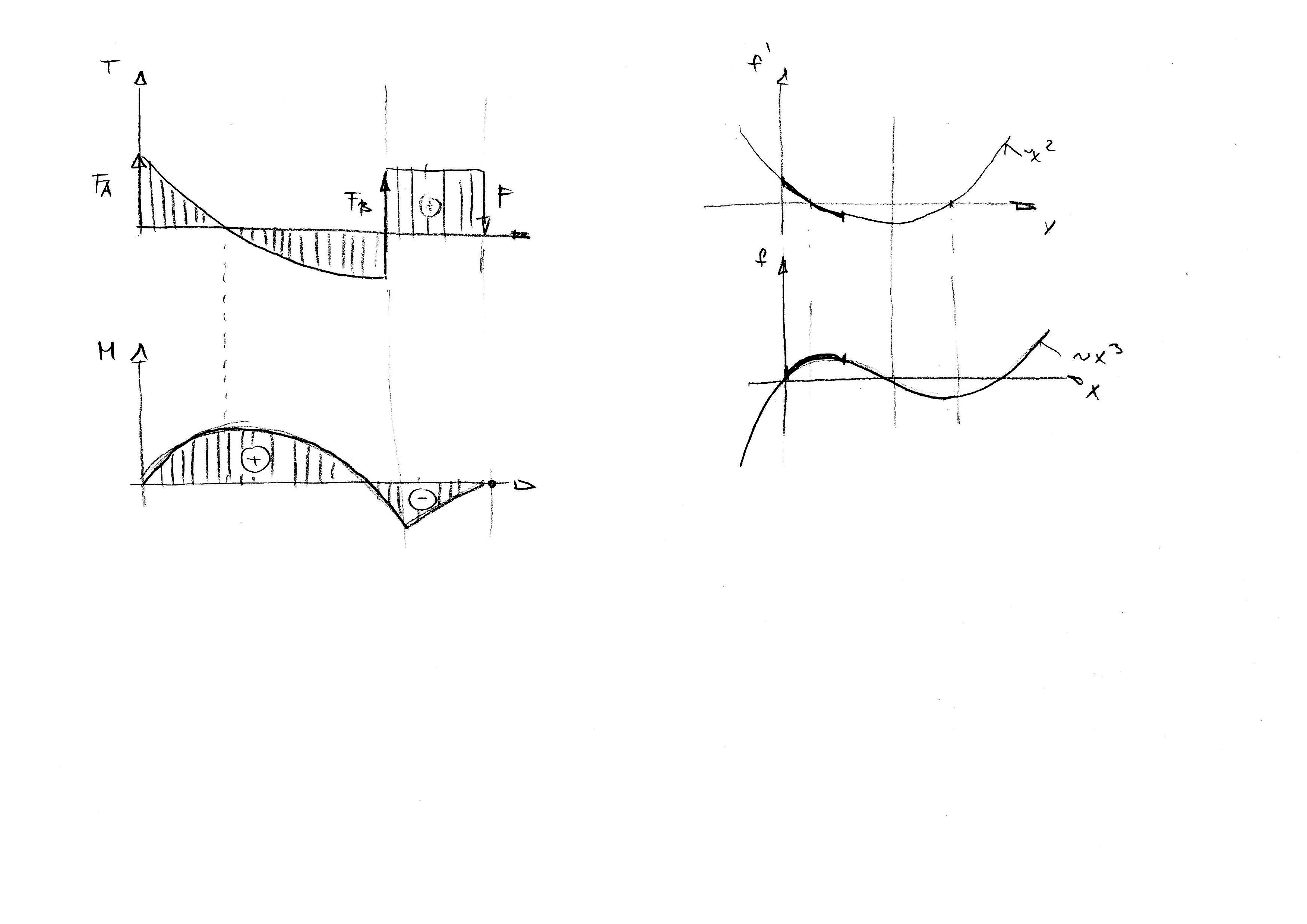
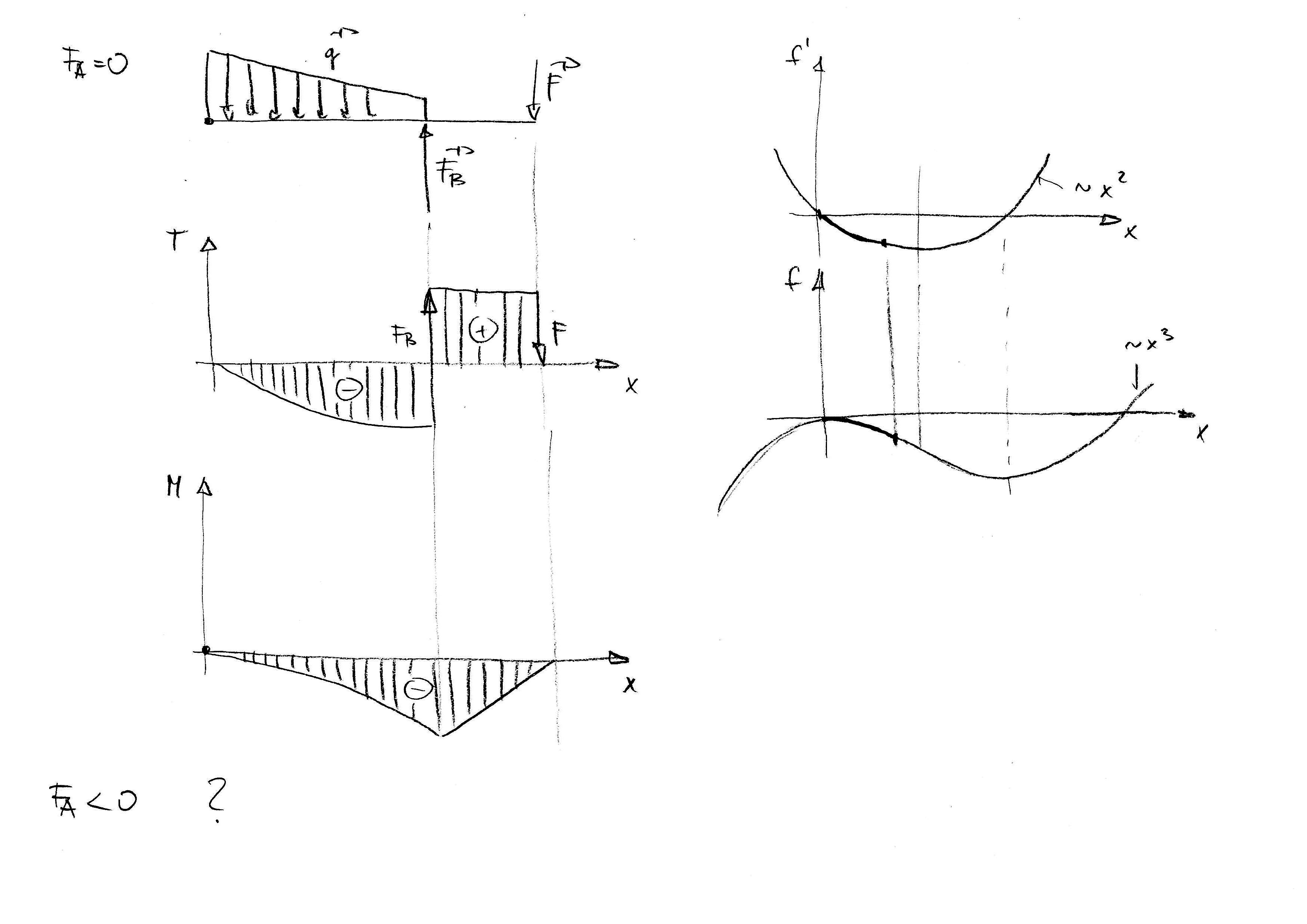
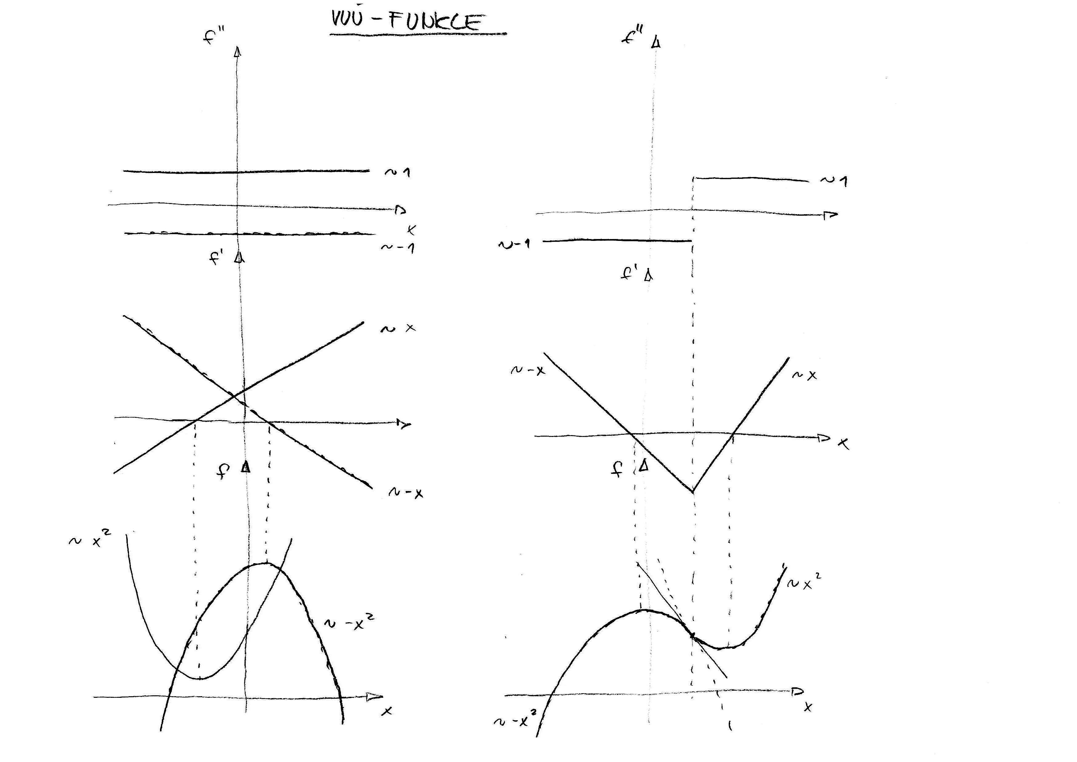
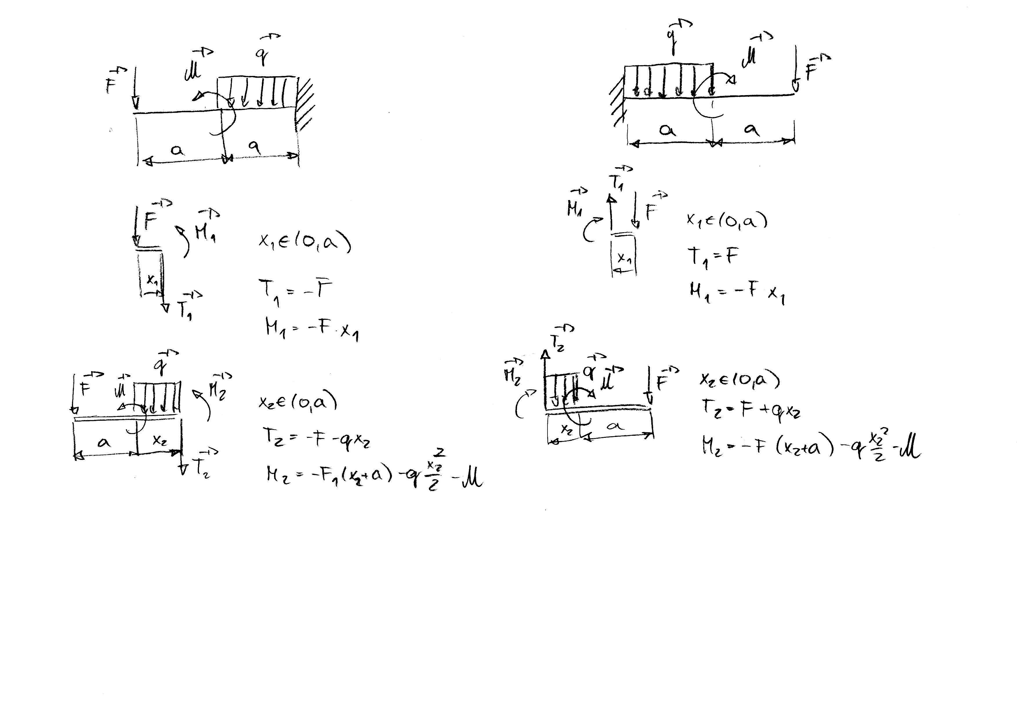
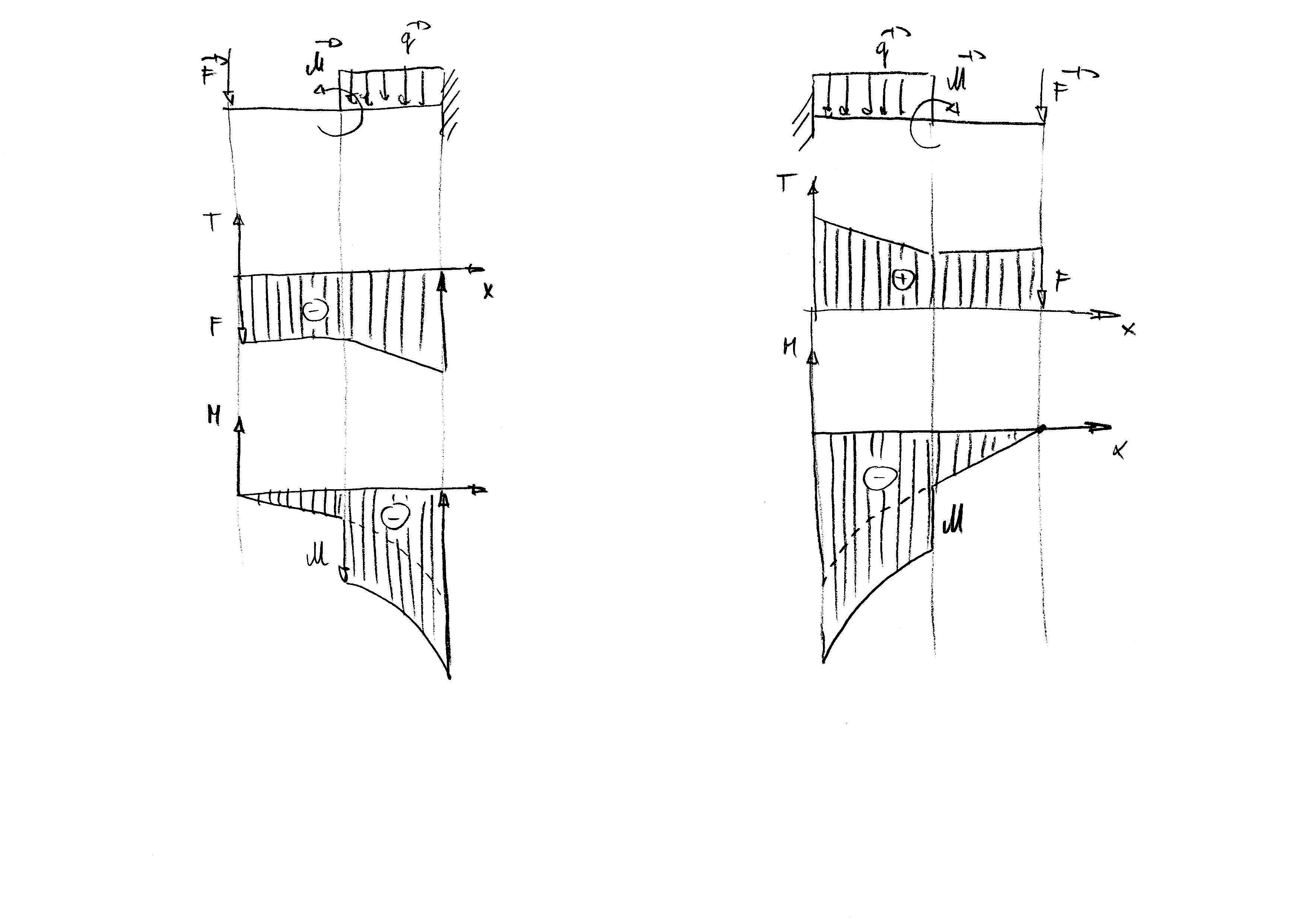
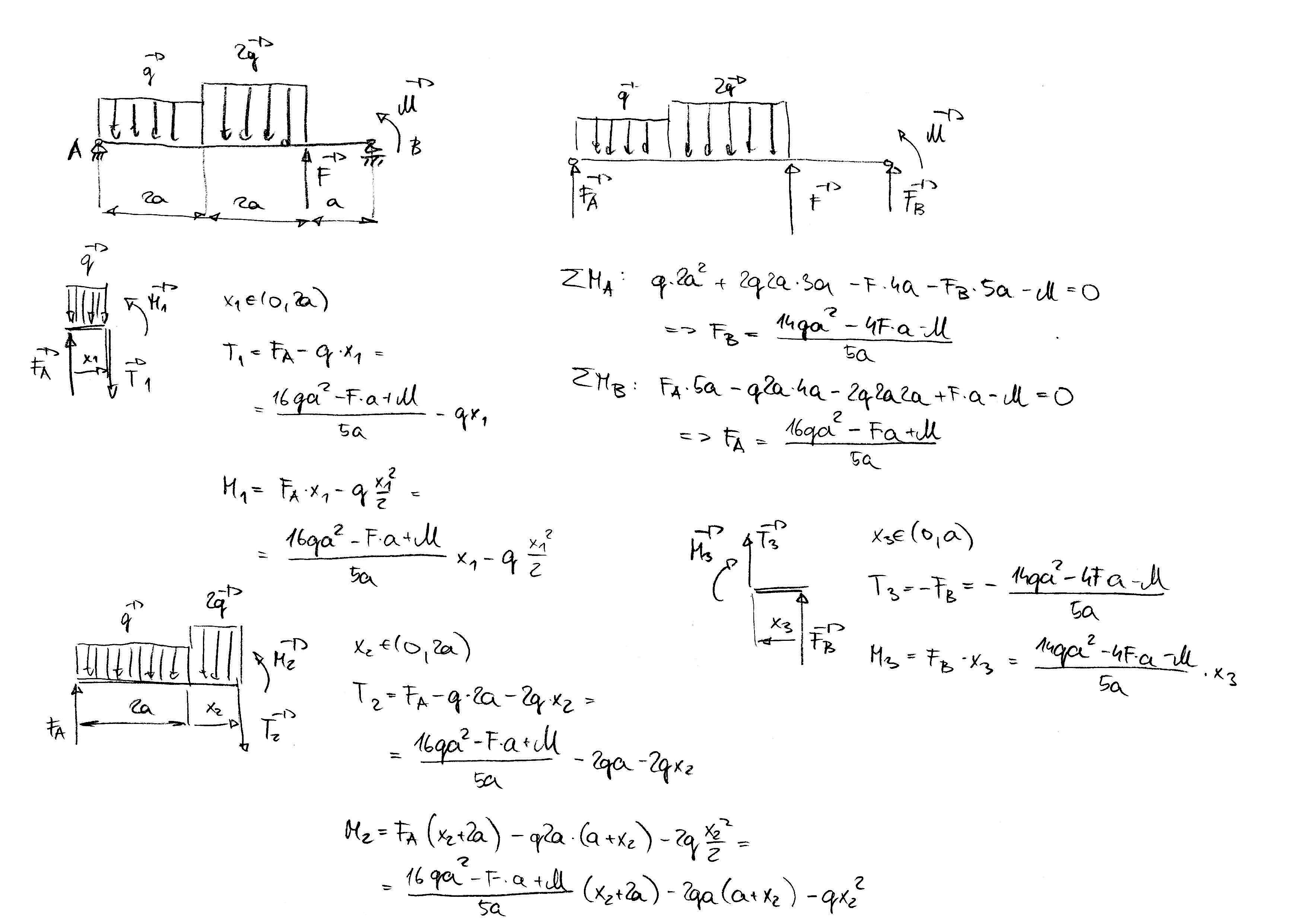
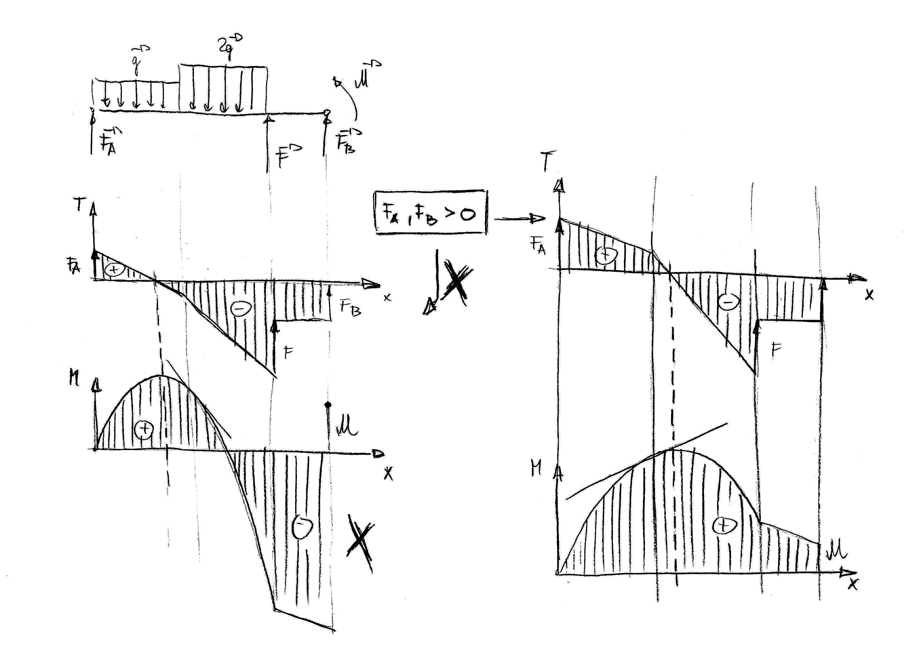
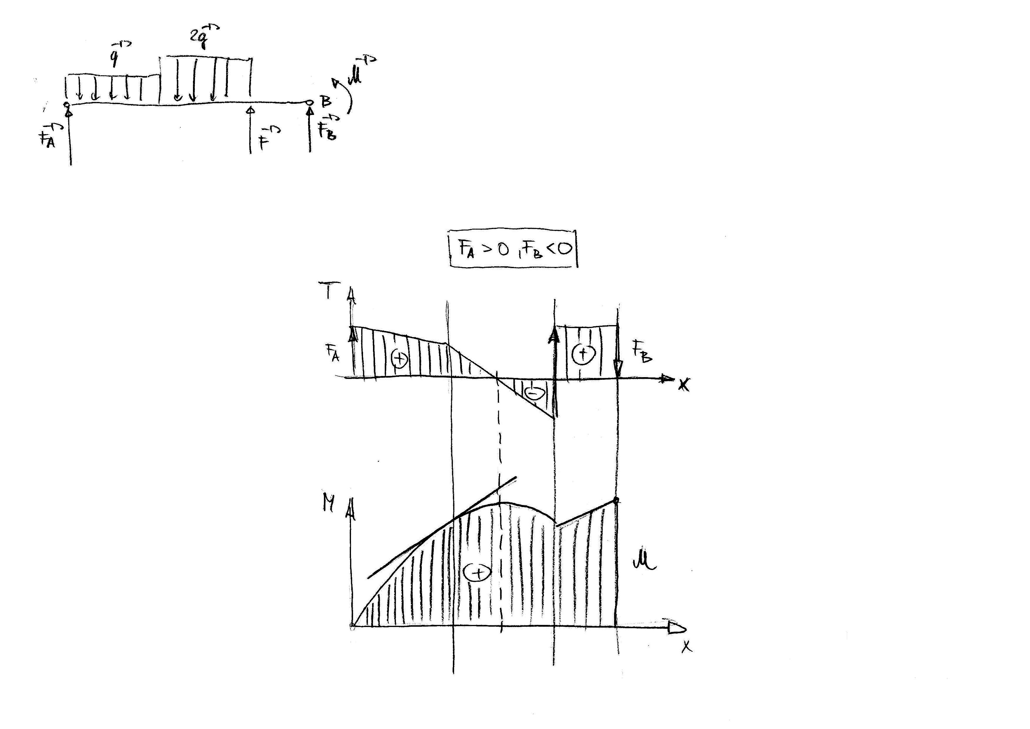
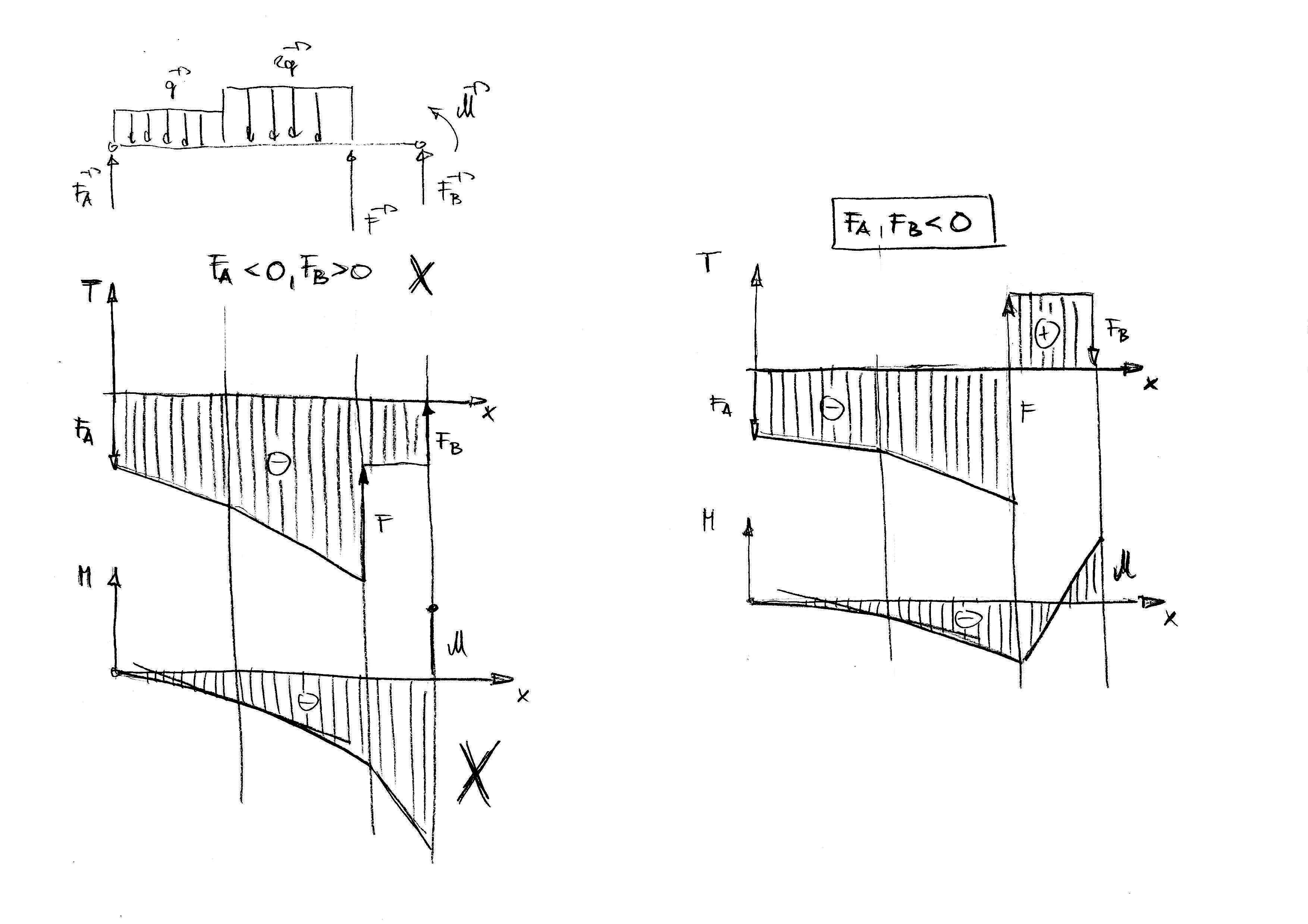
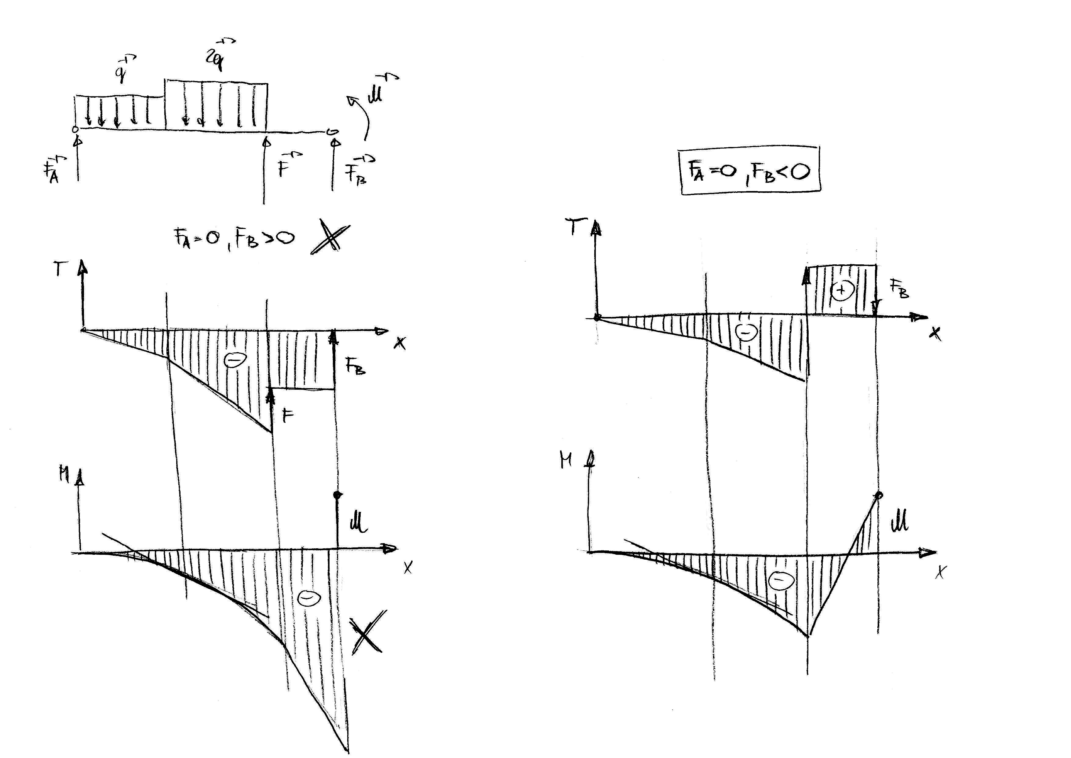
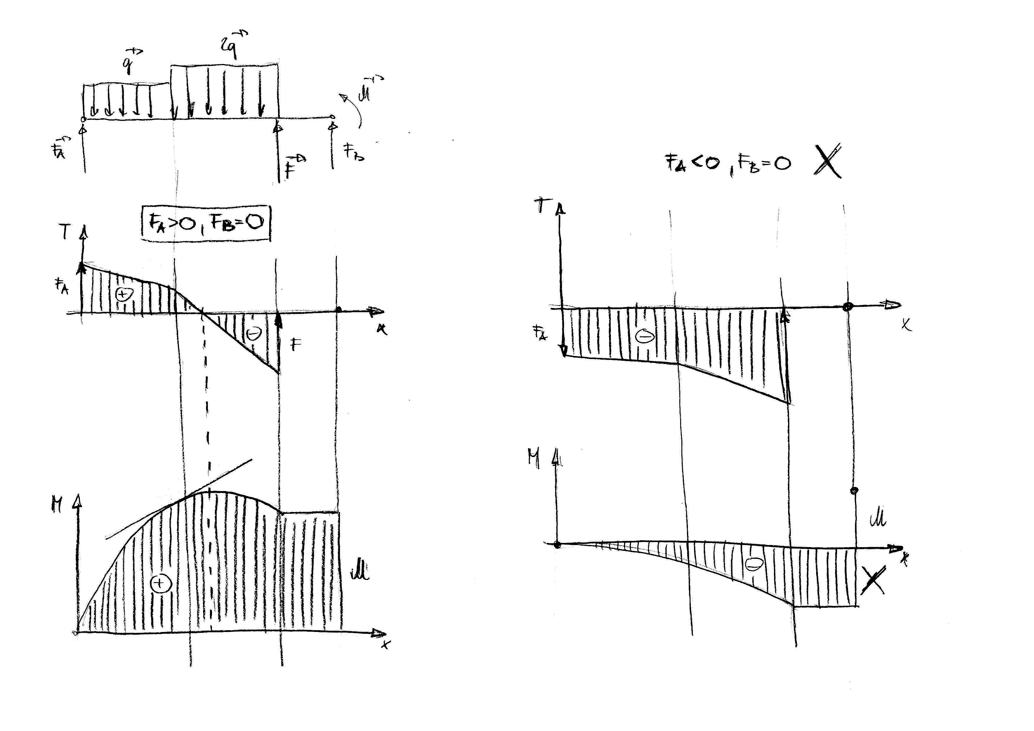
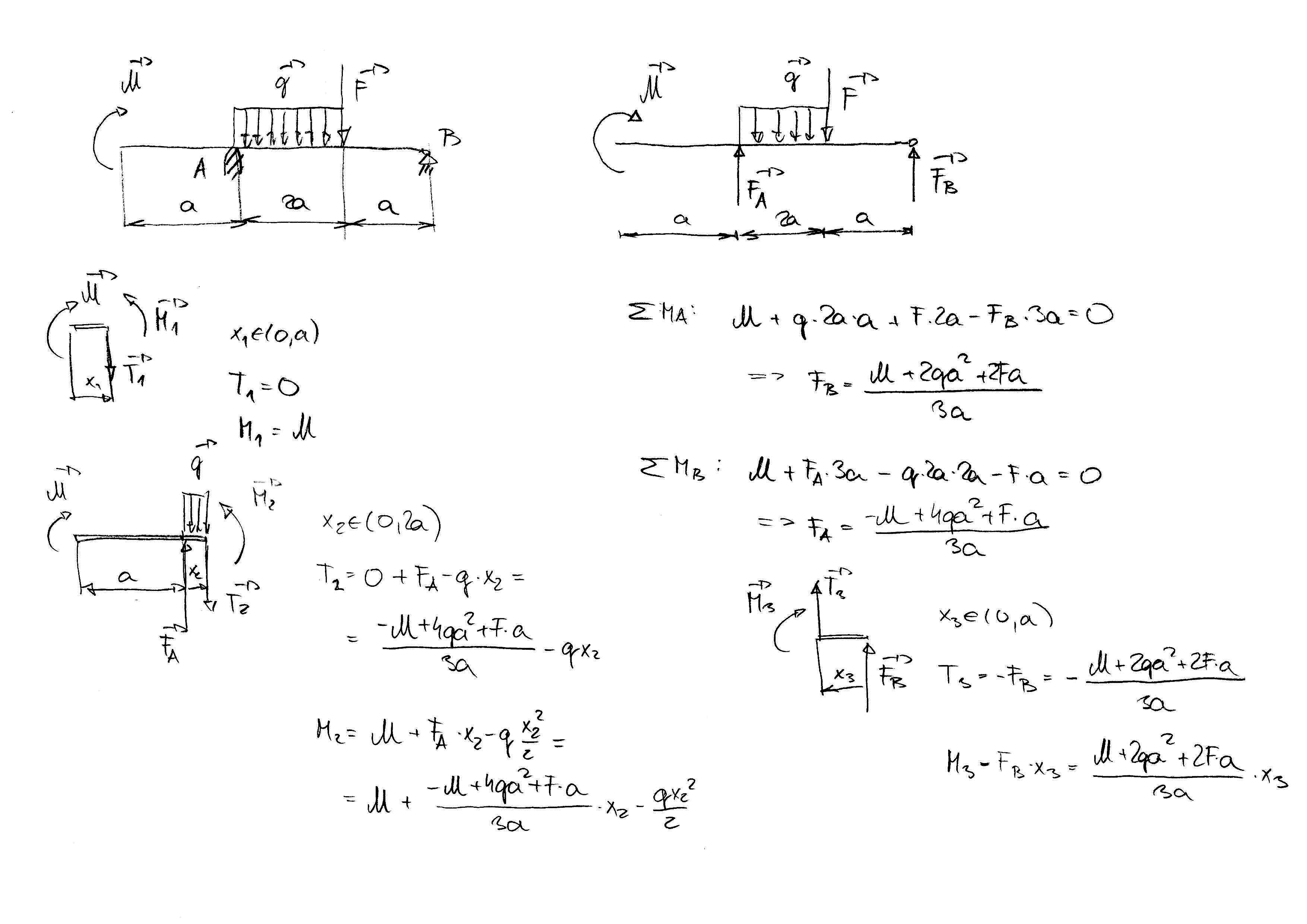
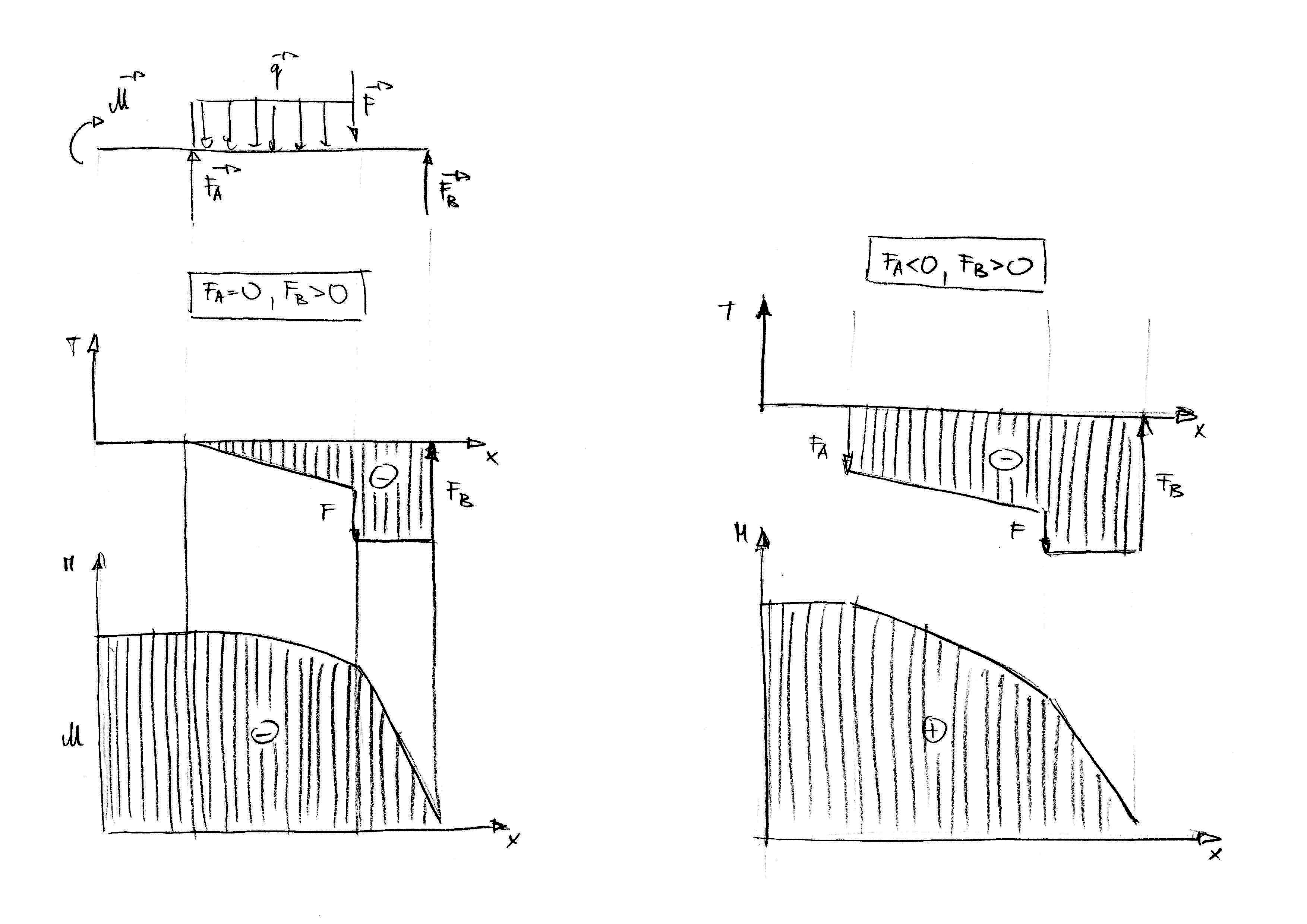
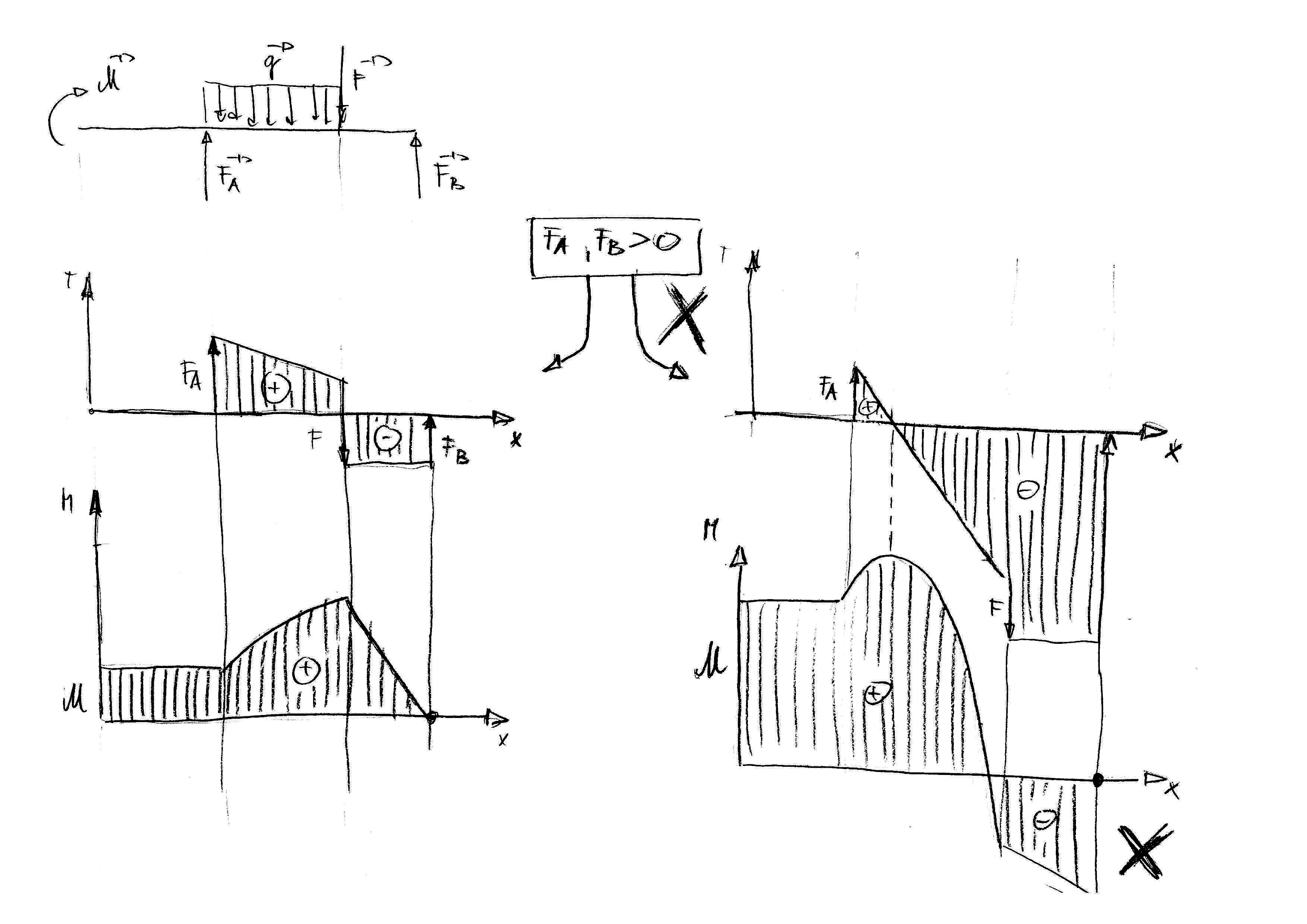
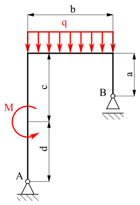
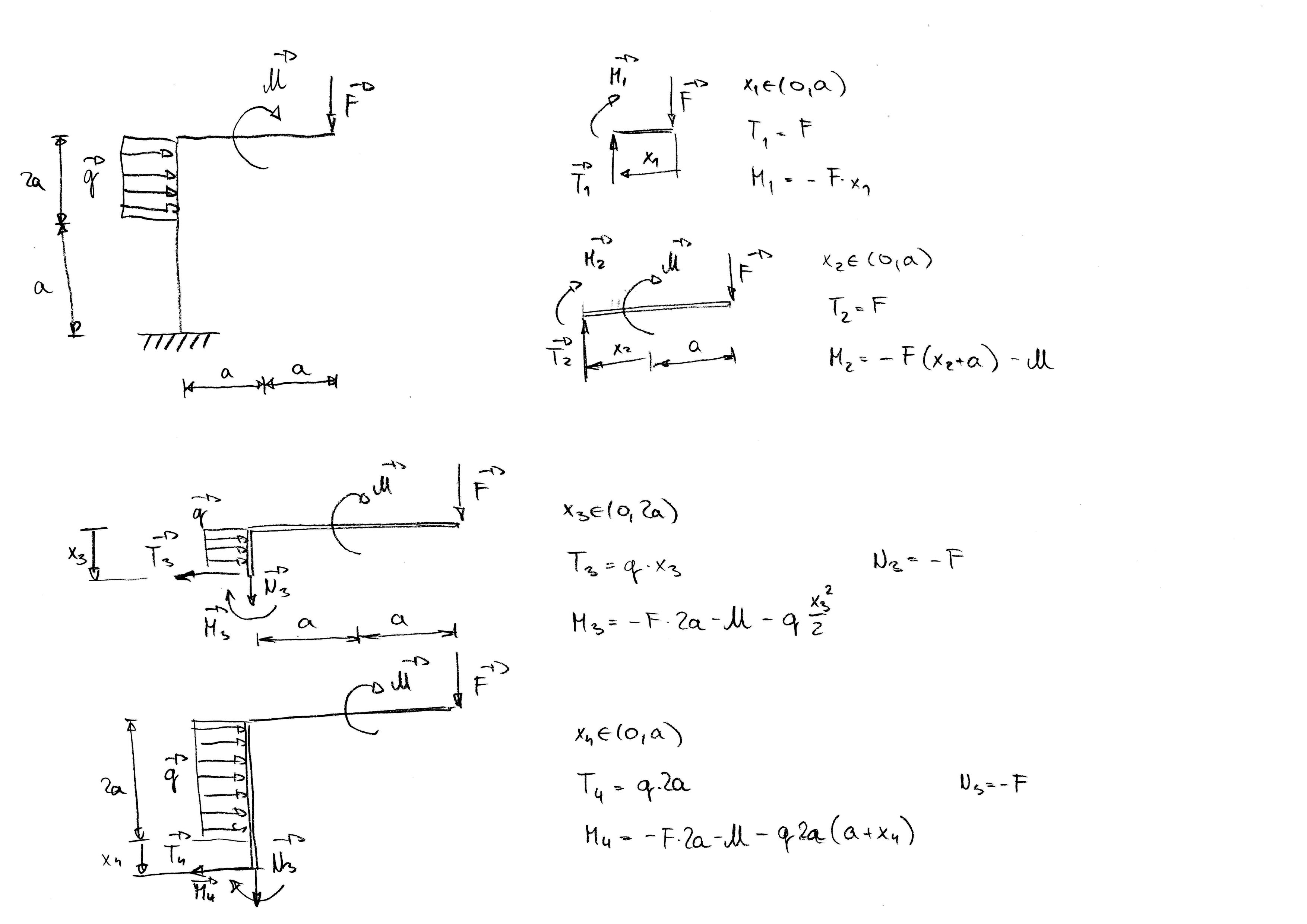
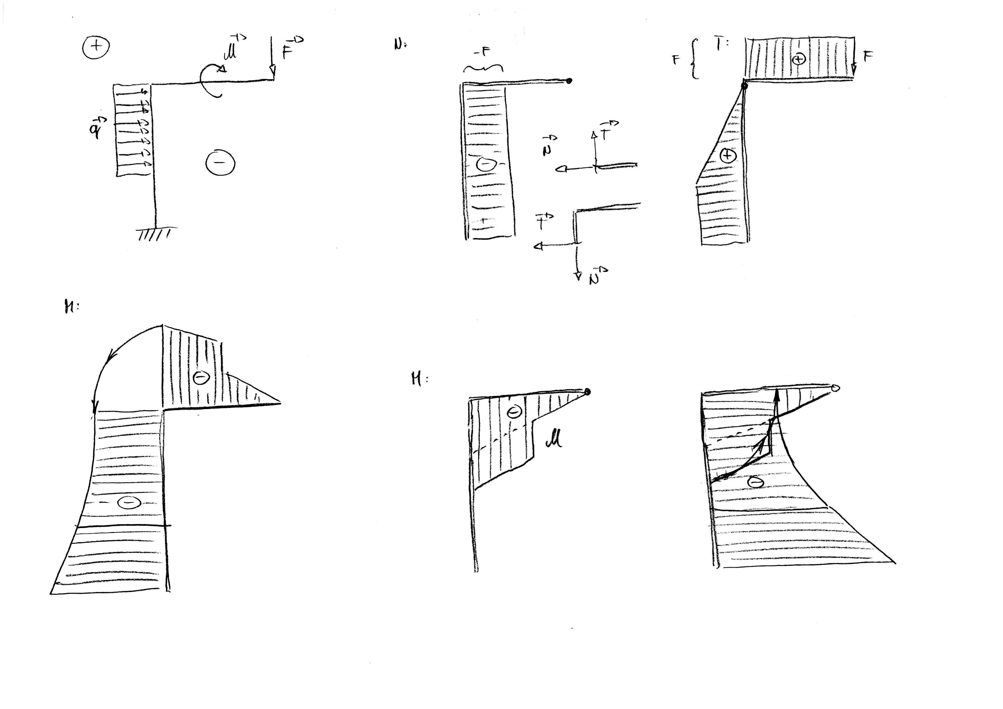
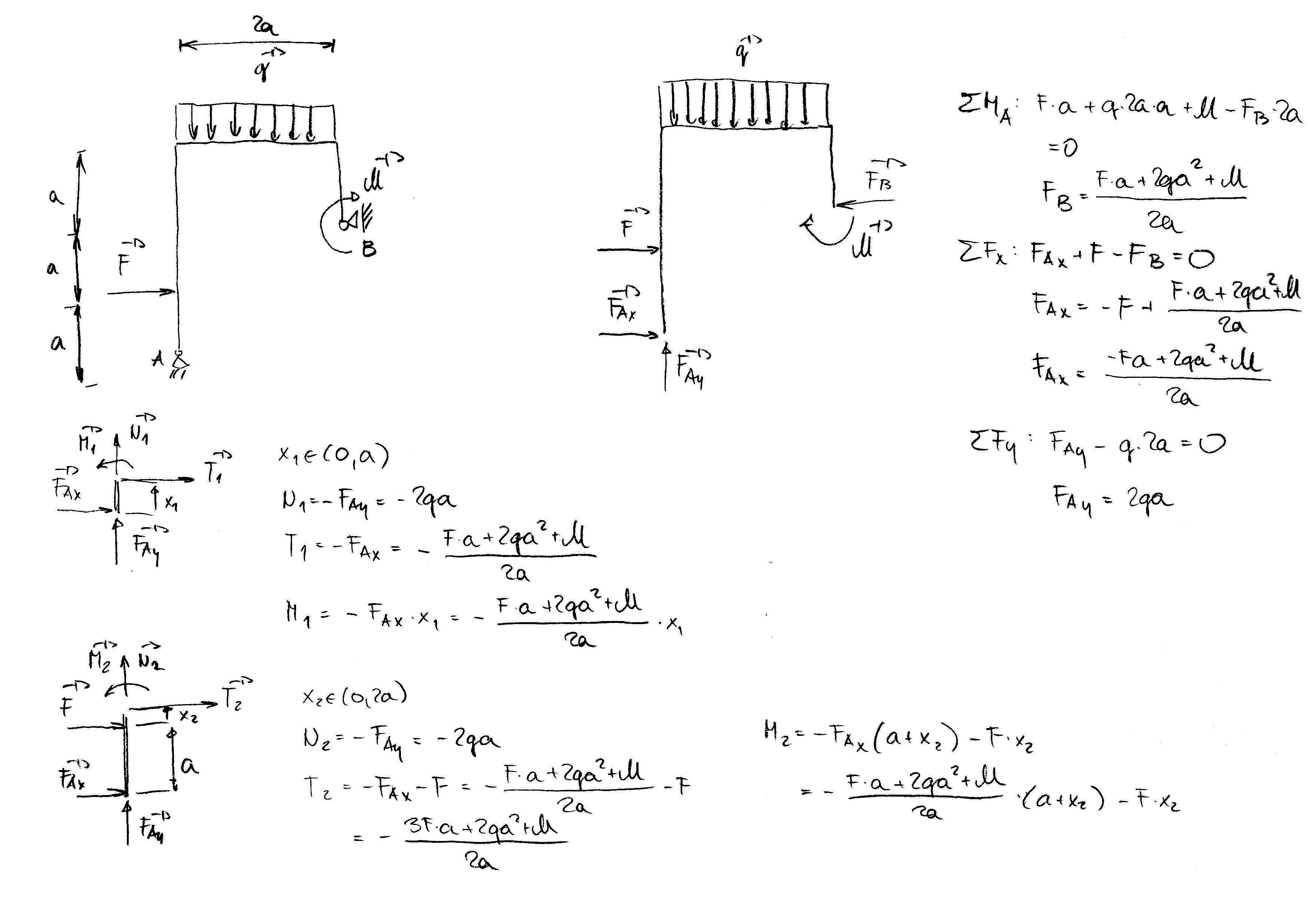
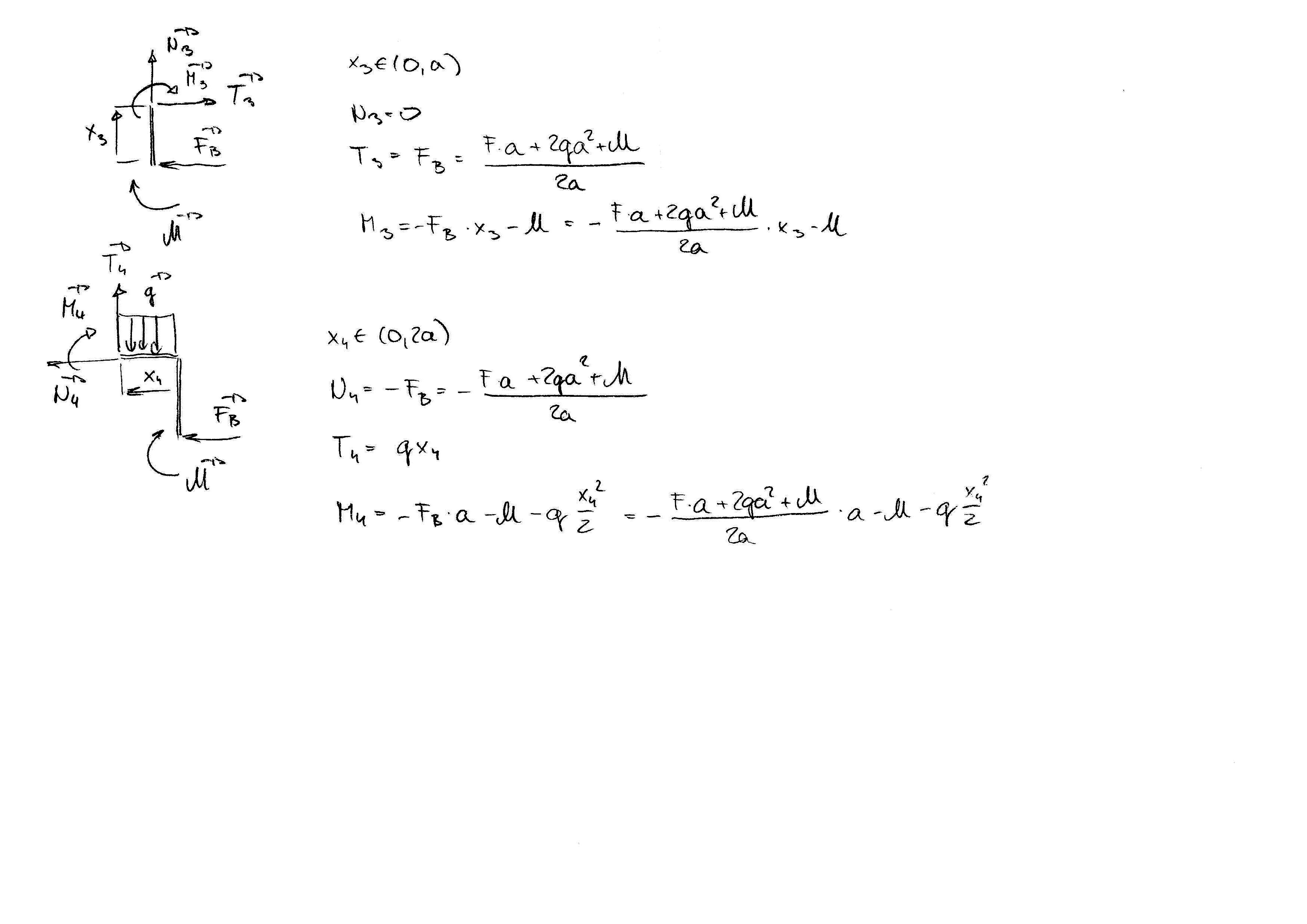
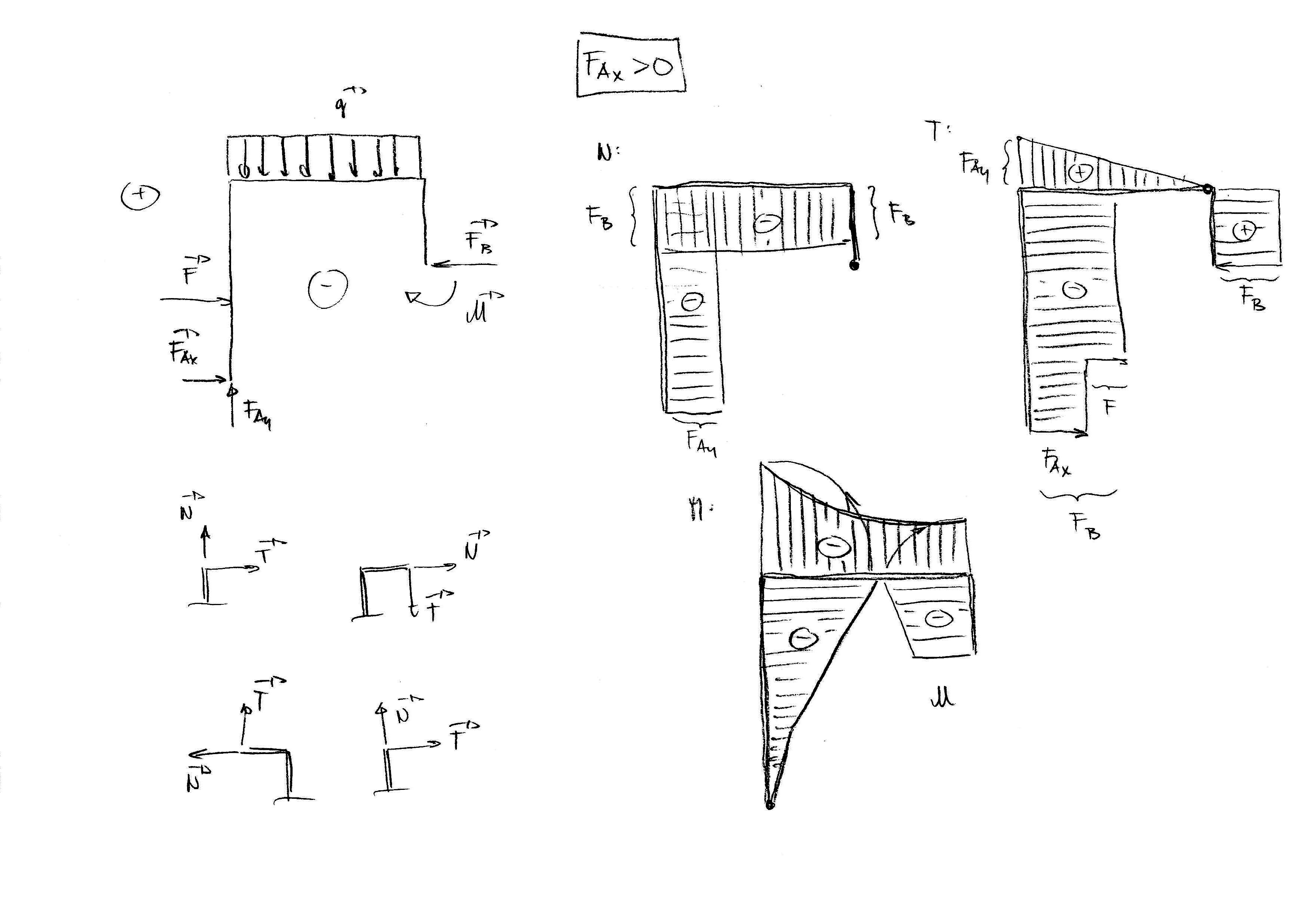
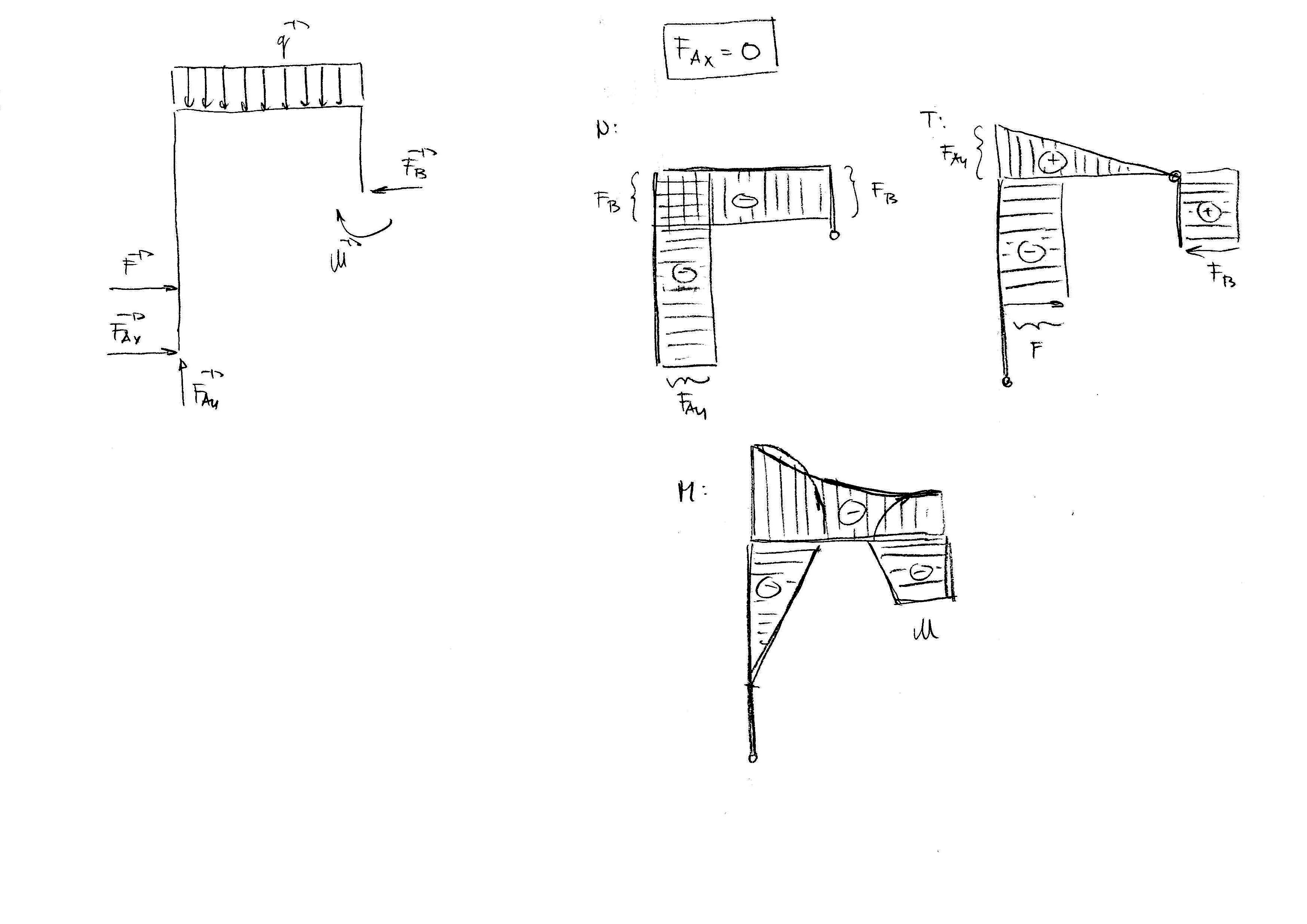
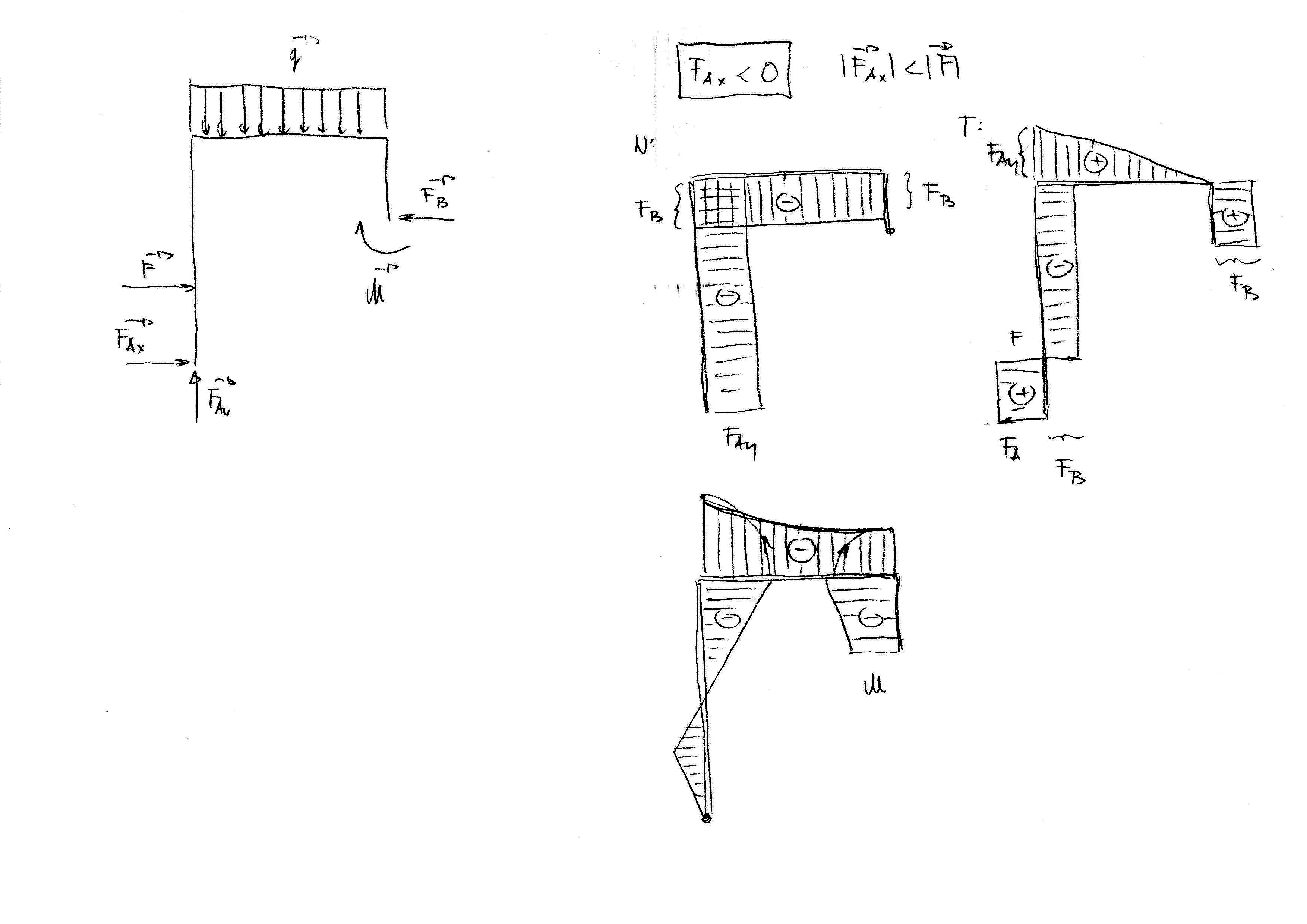
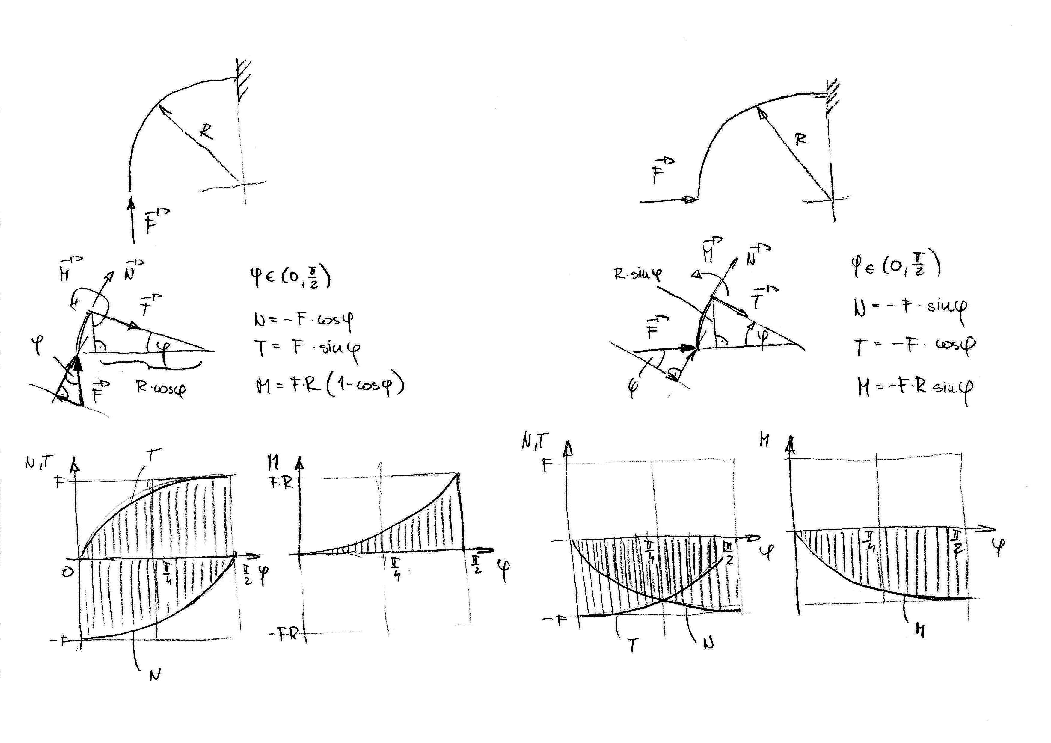
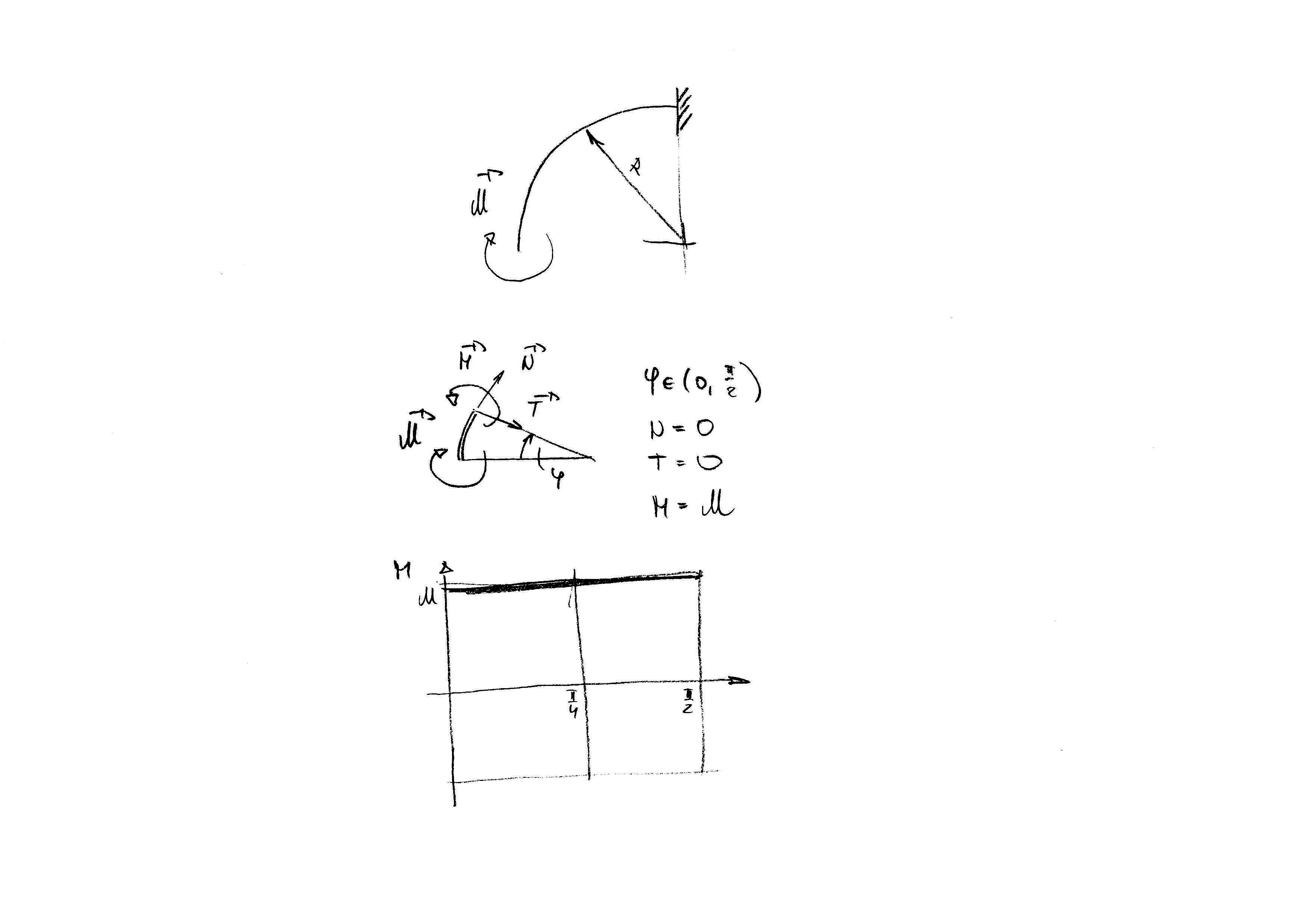
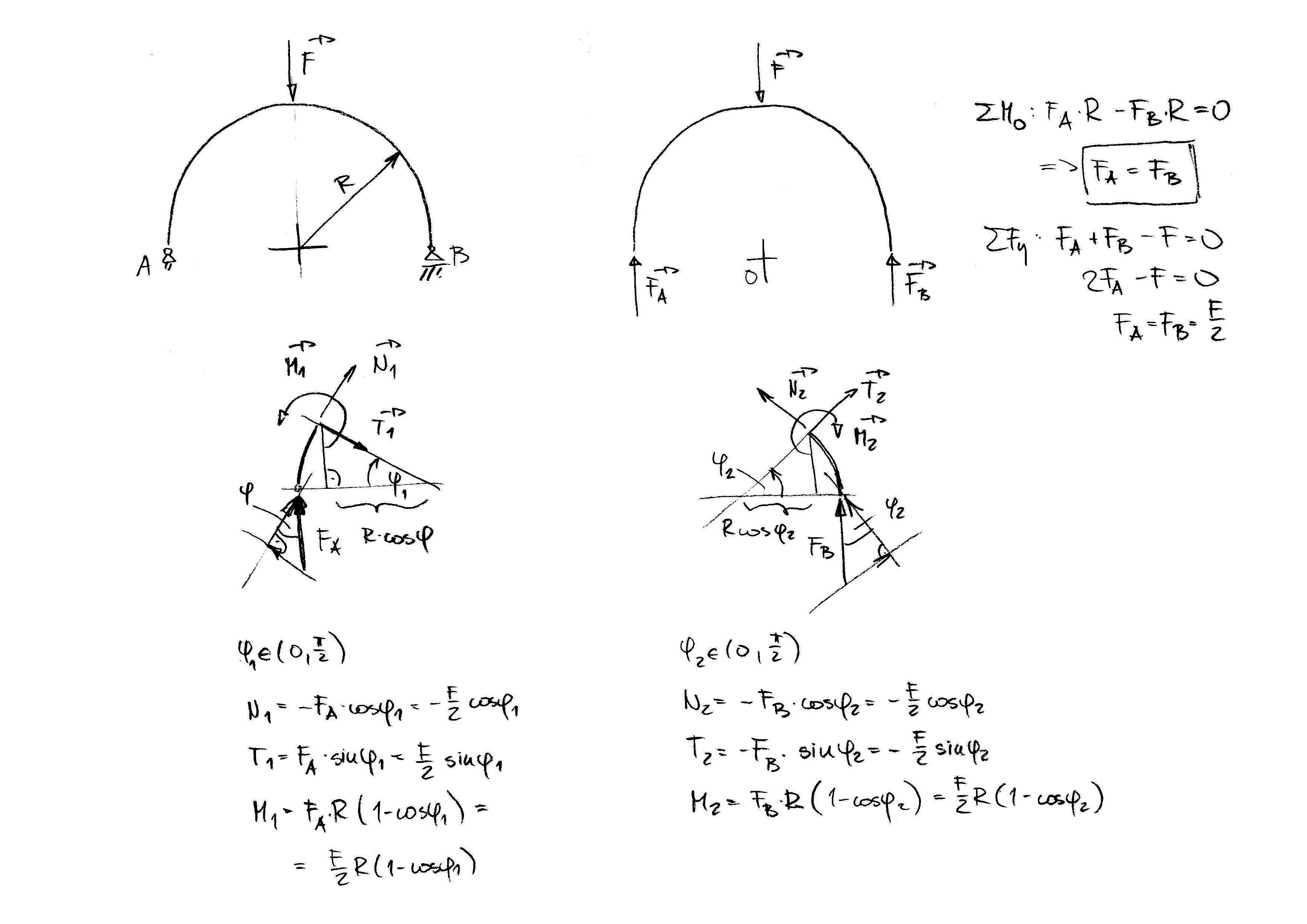
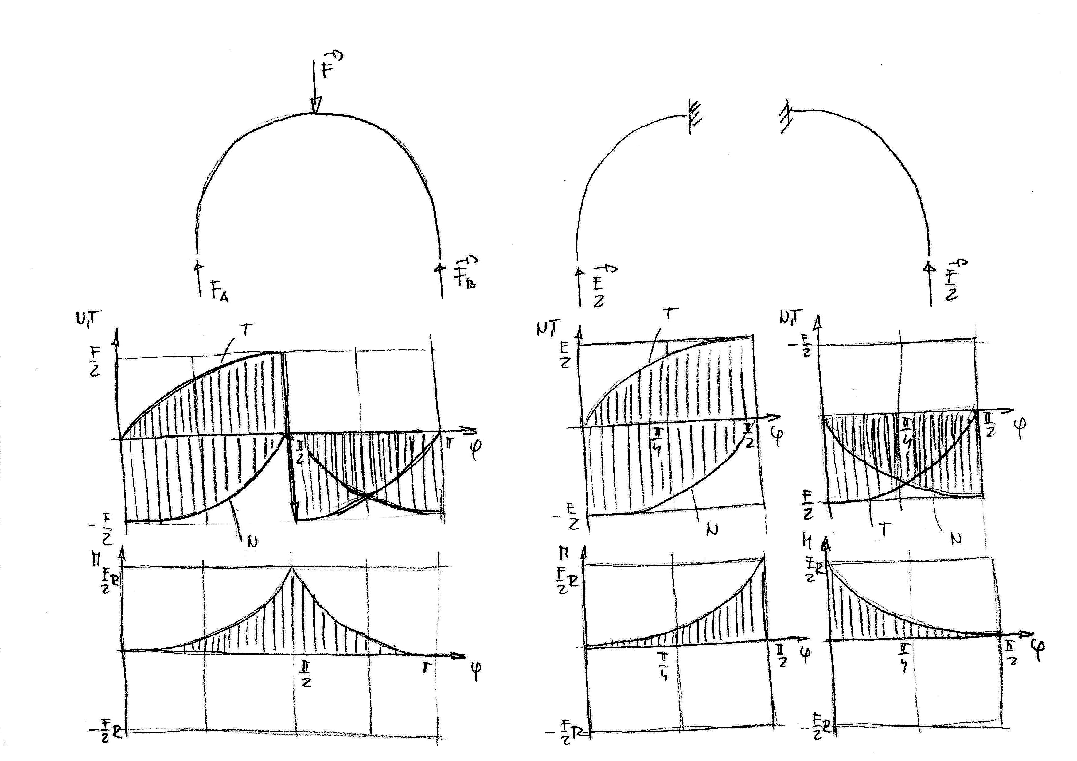
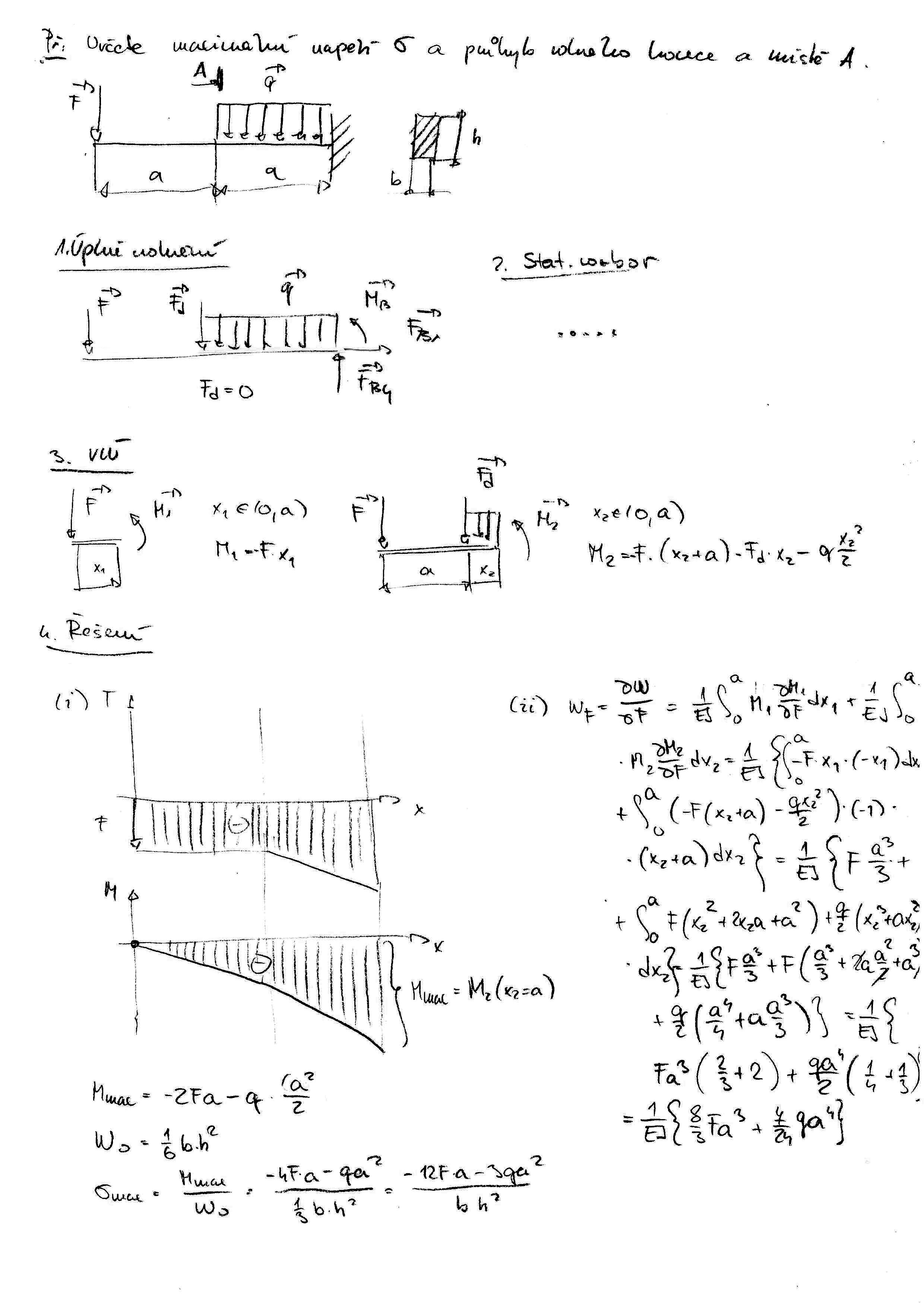
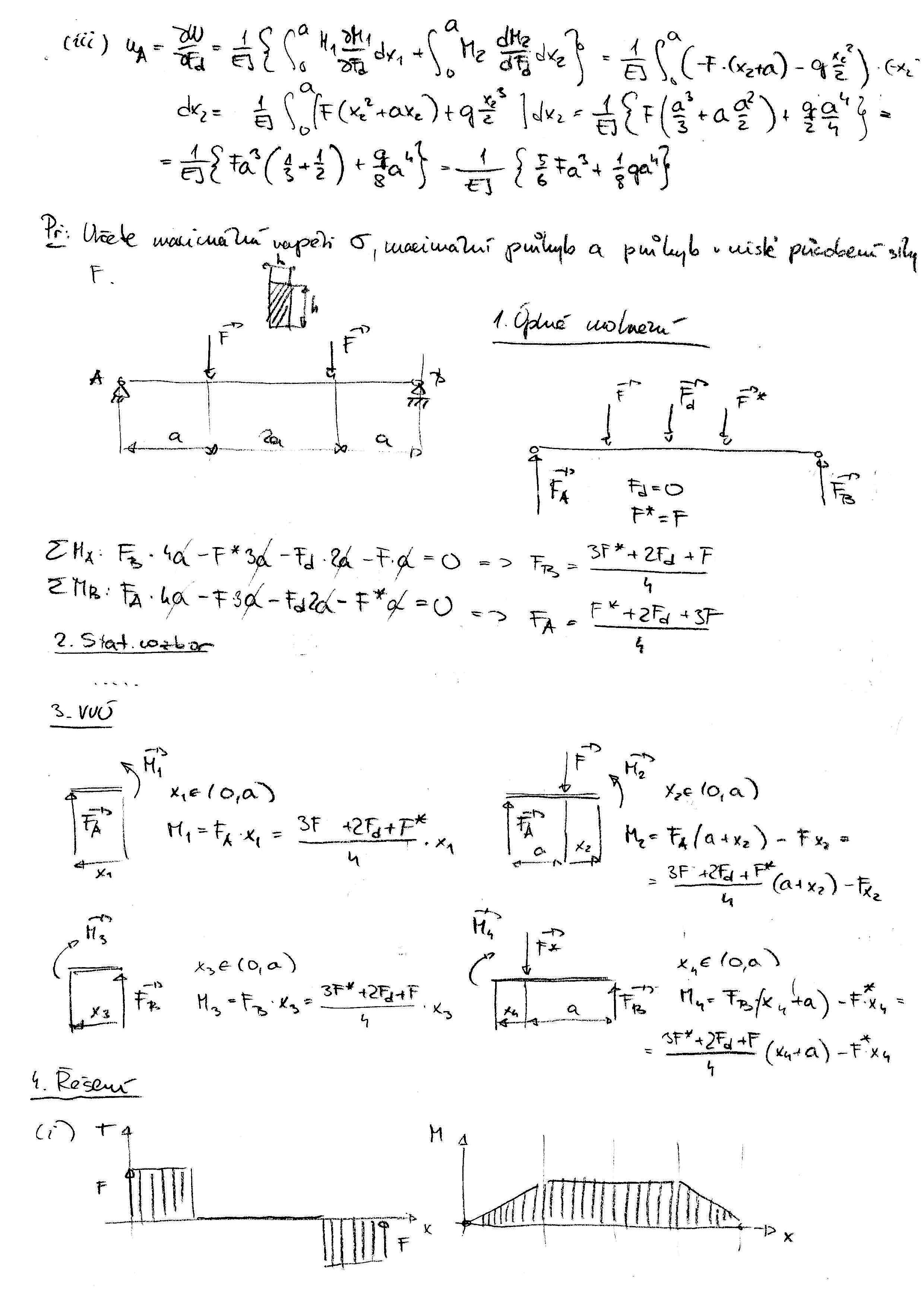
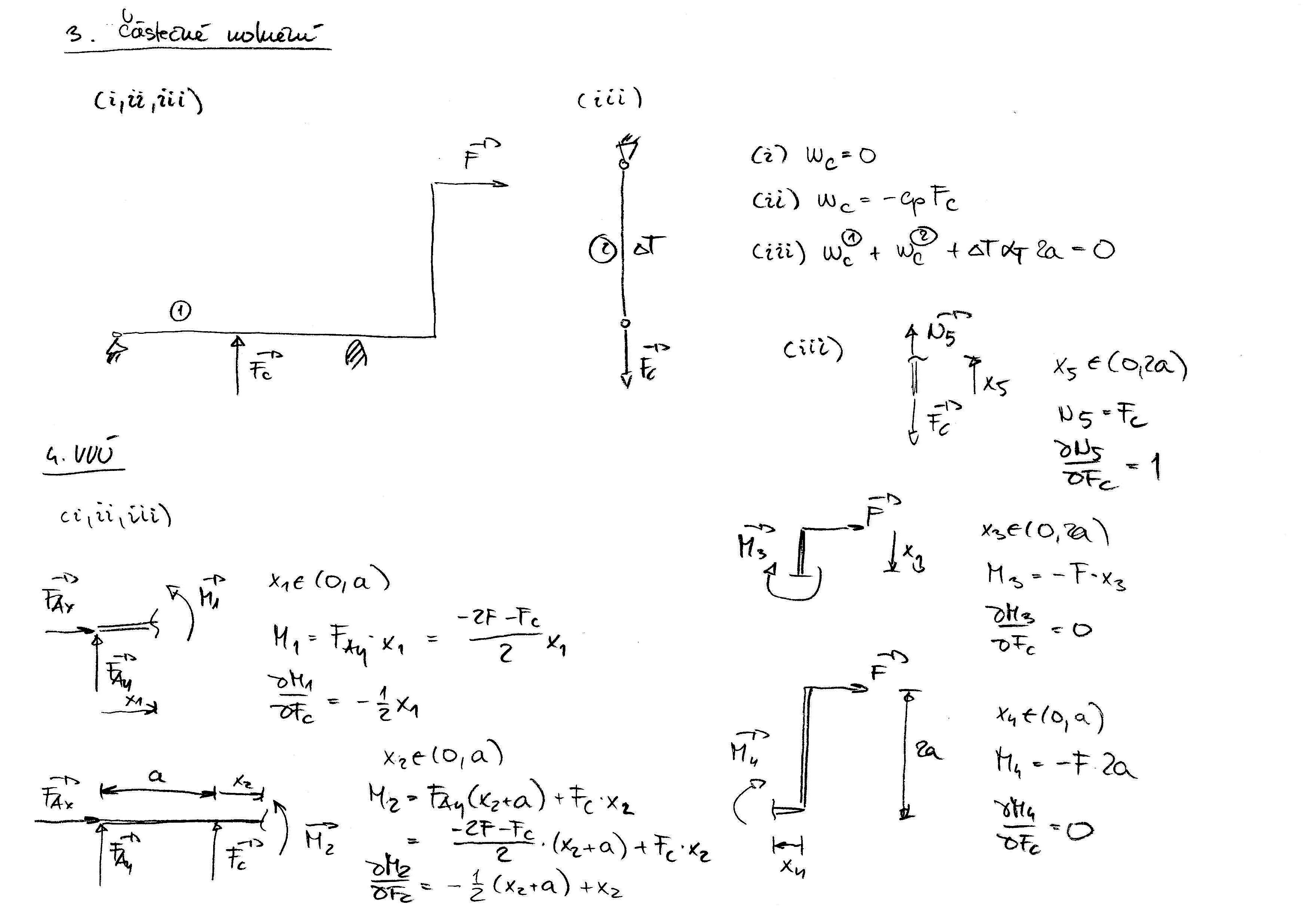
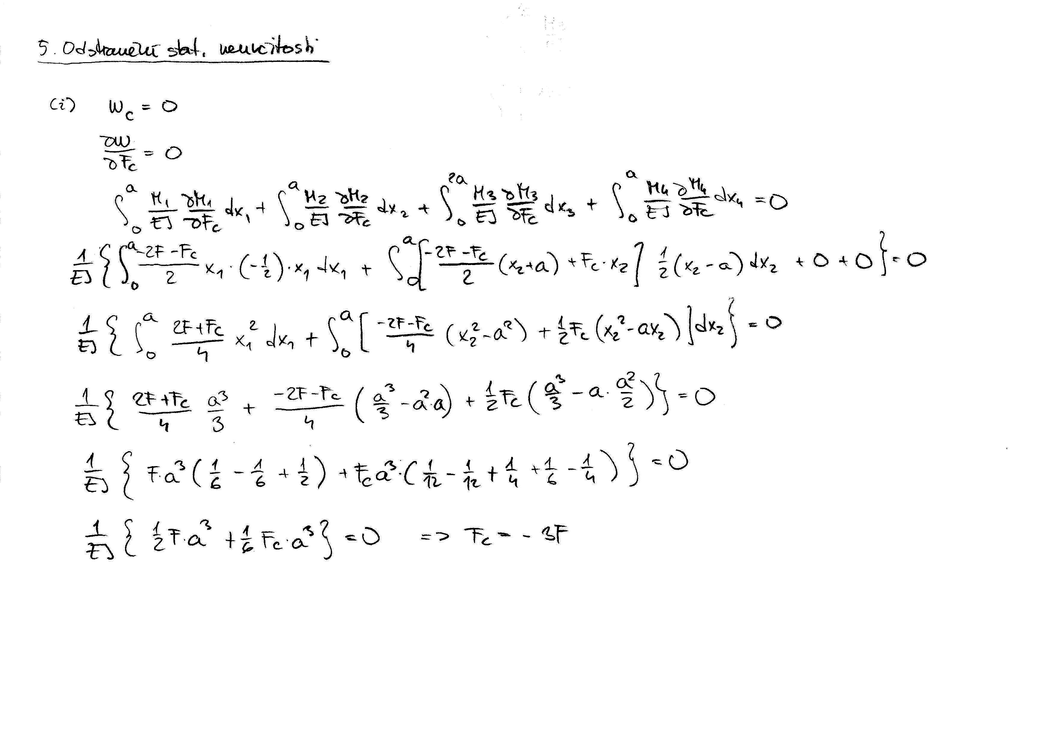
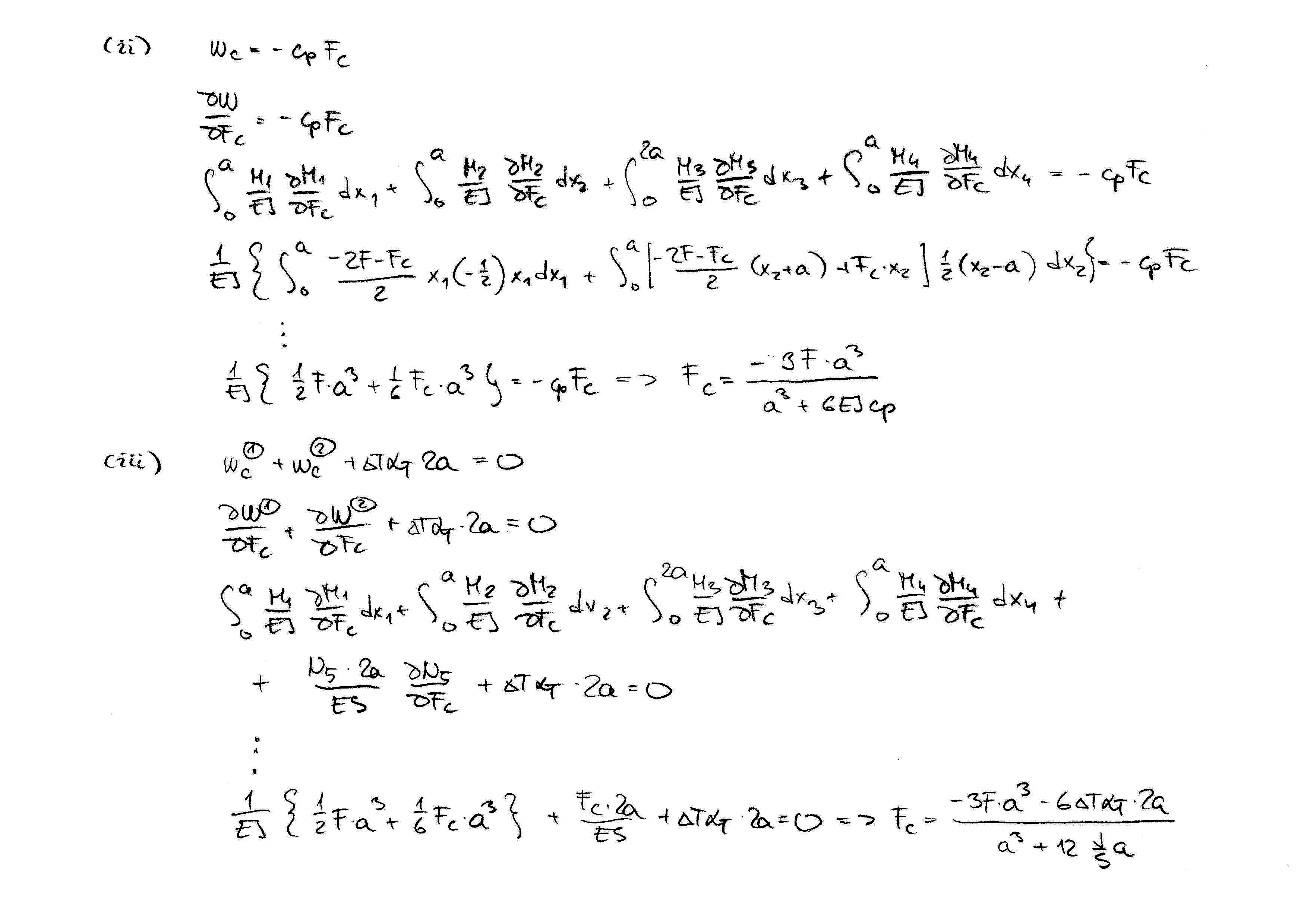
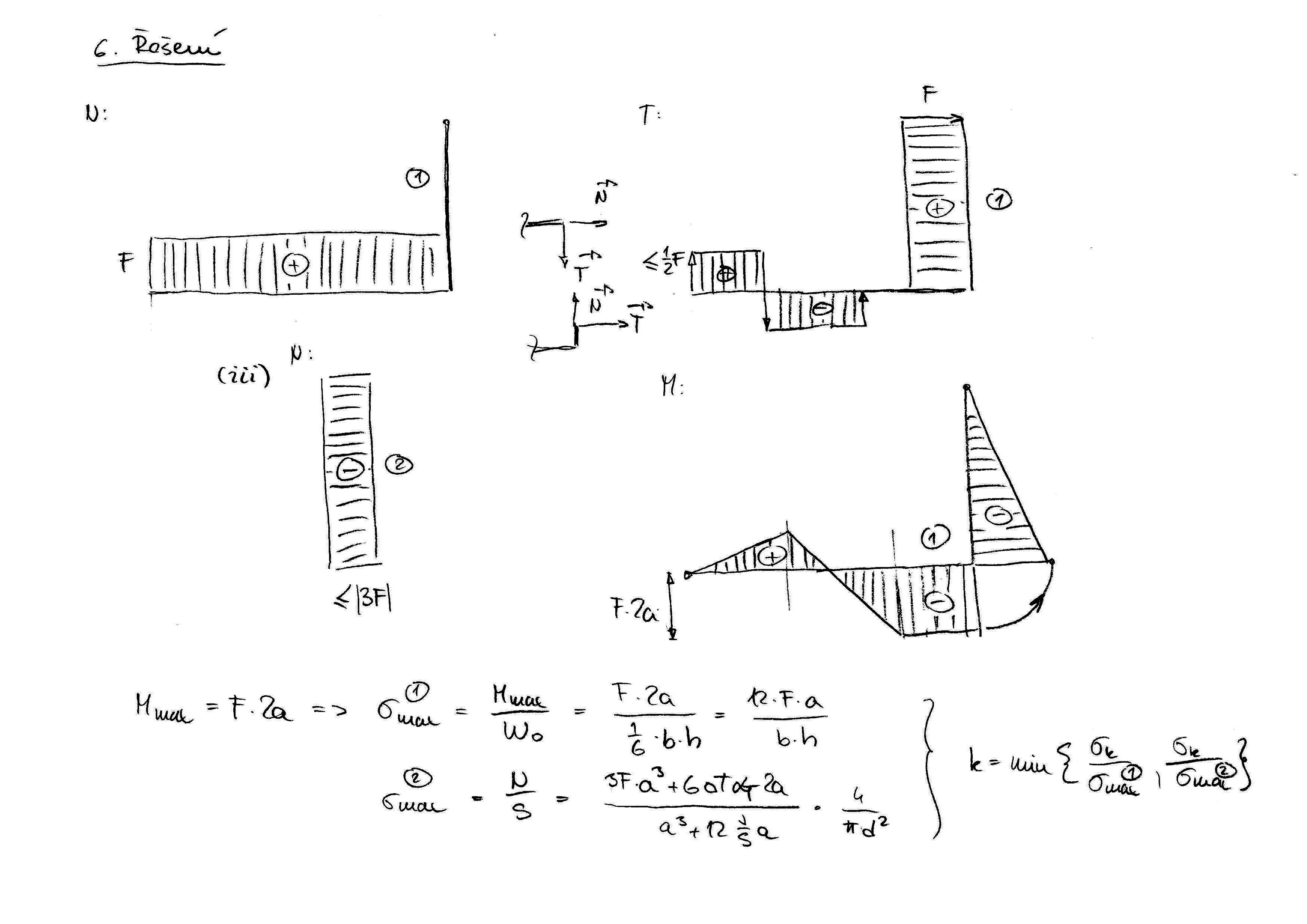
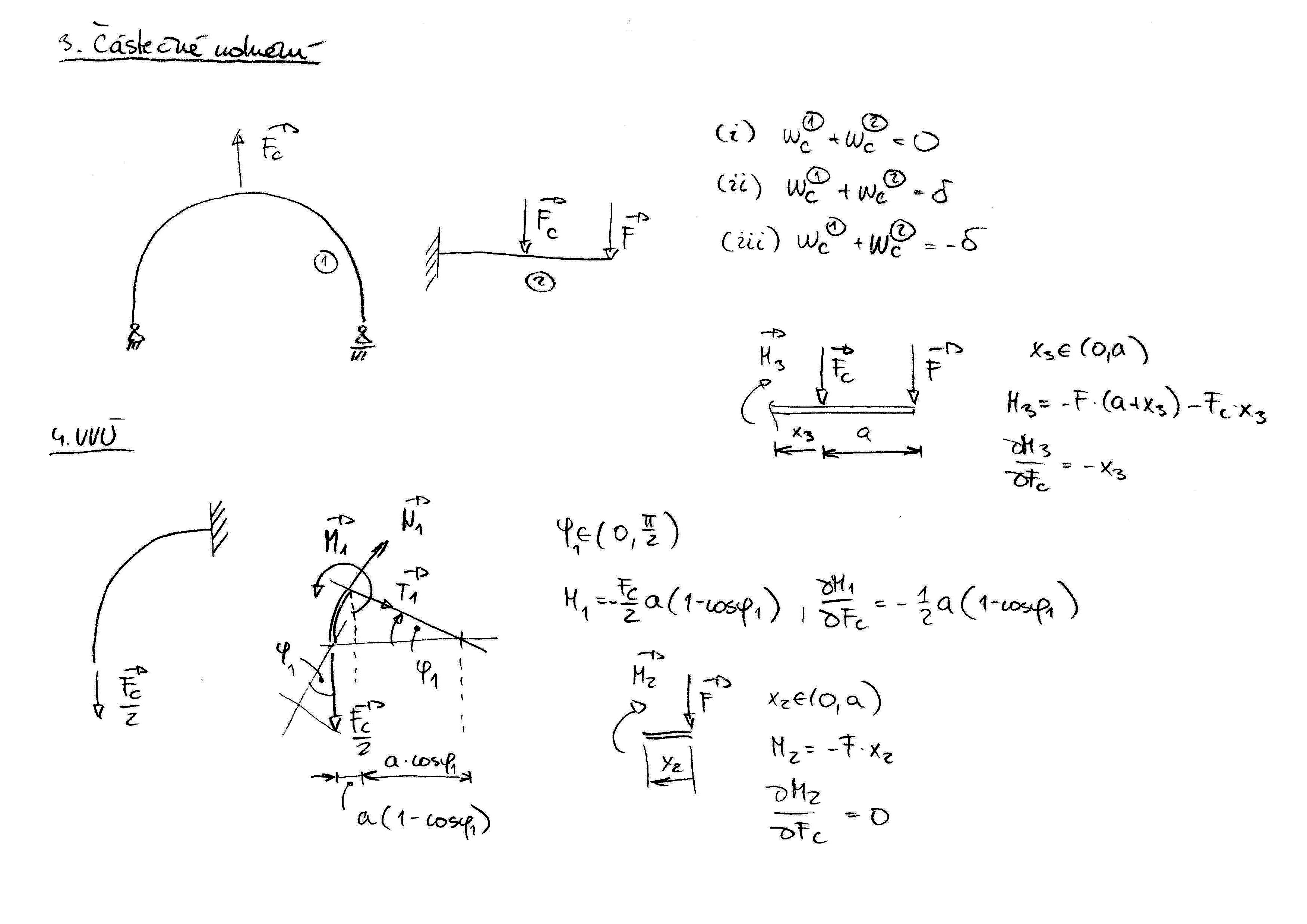
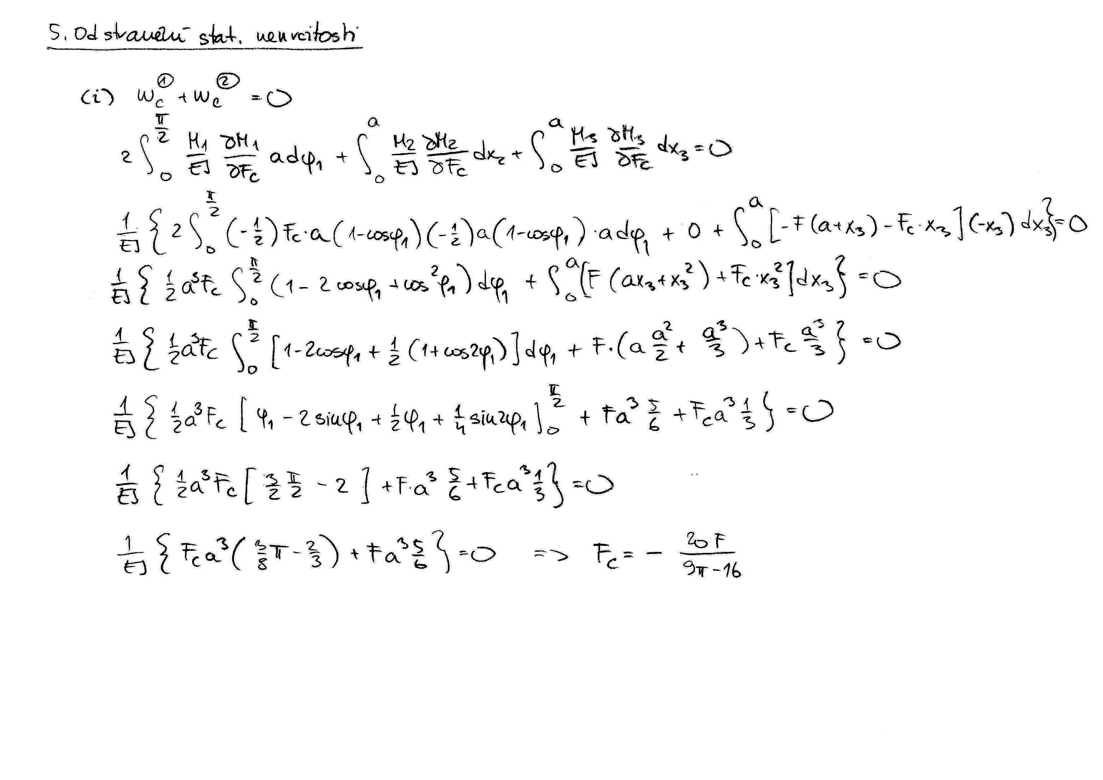
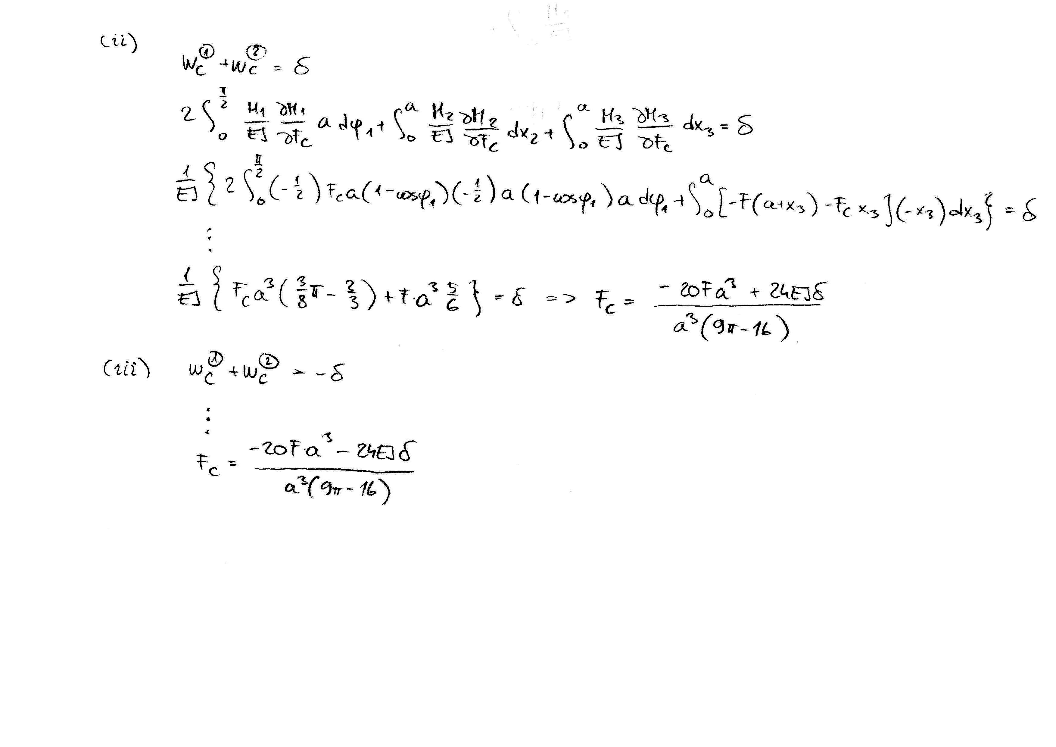
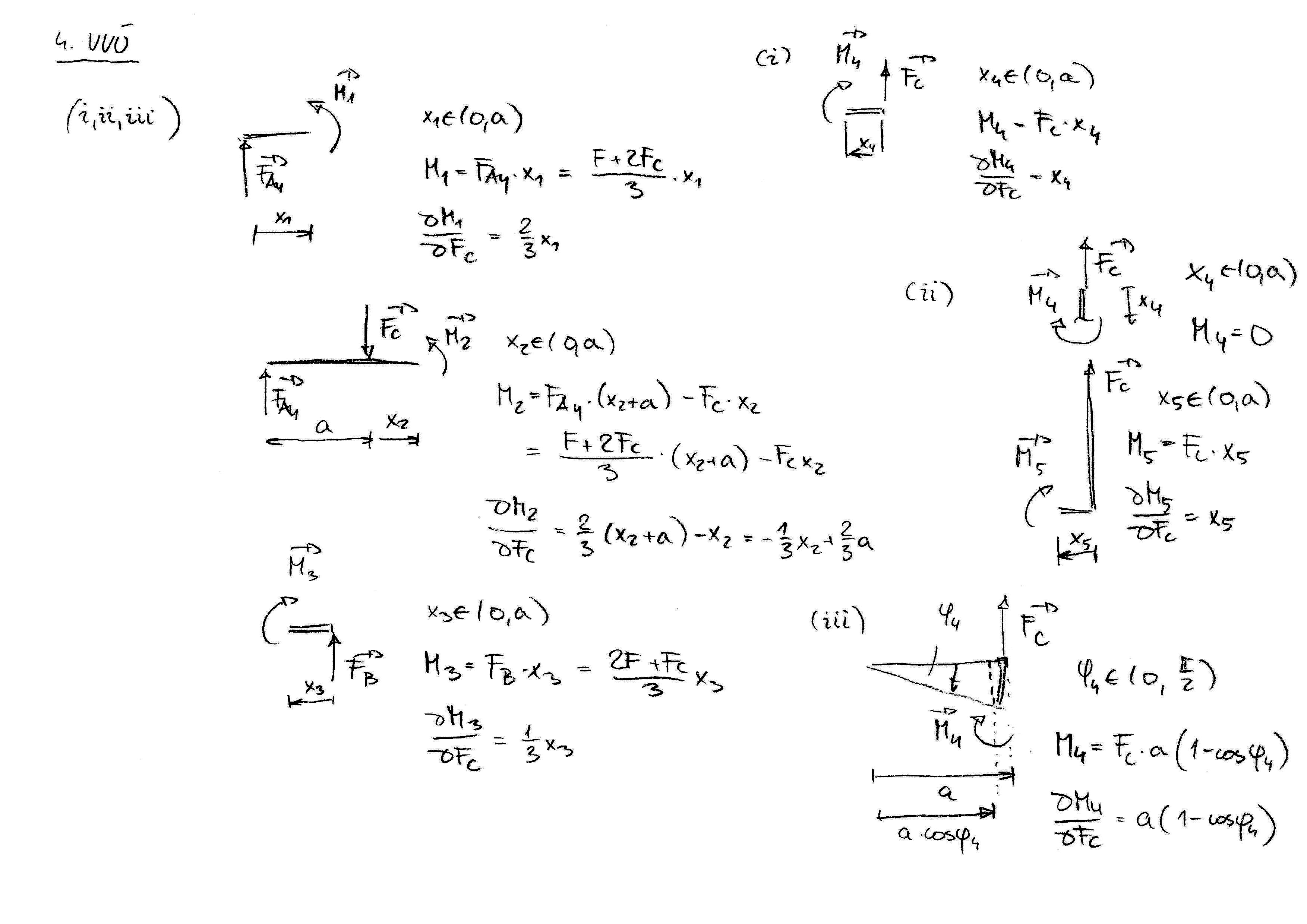
  • Cvičení 12: Výsledné vnitřní účinky (VVÚ)

Pružnost a pevnost I

Ukázkové příklady k procvičení jsou ve formátu *.ipynb. Jde o soubory použitelné v systému Jupyter, který si můžete stáhnout na stránkách jupyter.org pro případ Pythonu nebo otestovat na stránce juliabox.com pro případ Julie, viz také ipython.org a julialang.org.

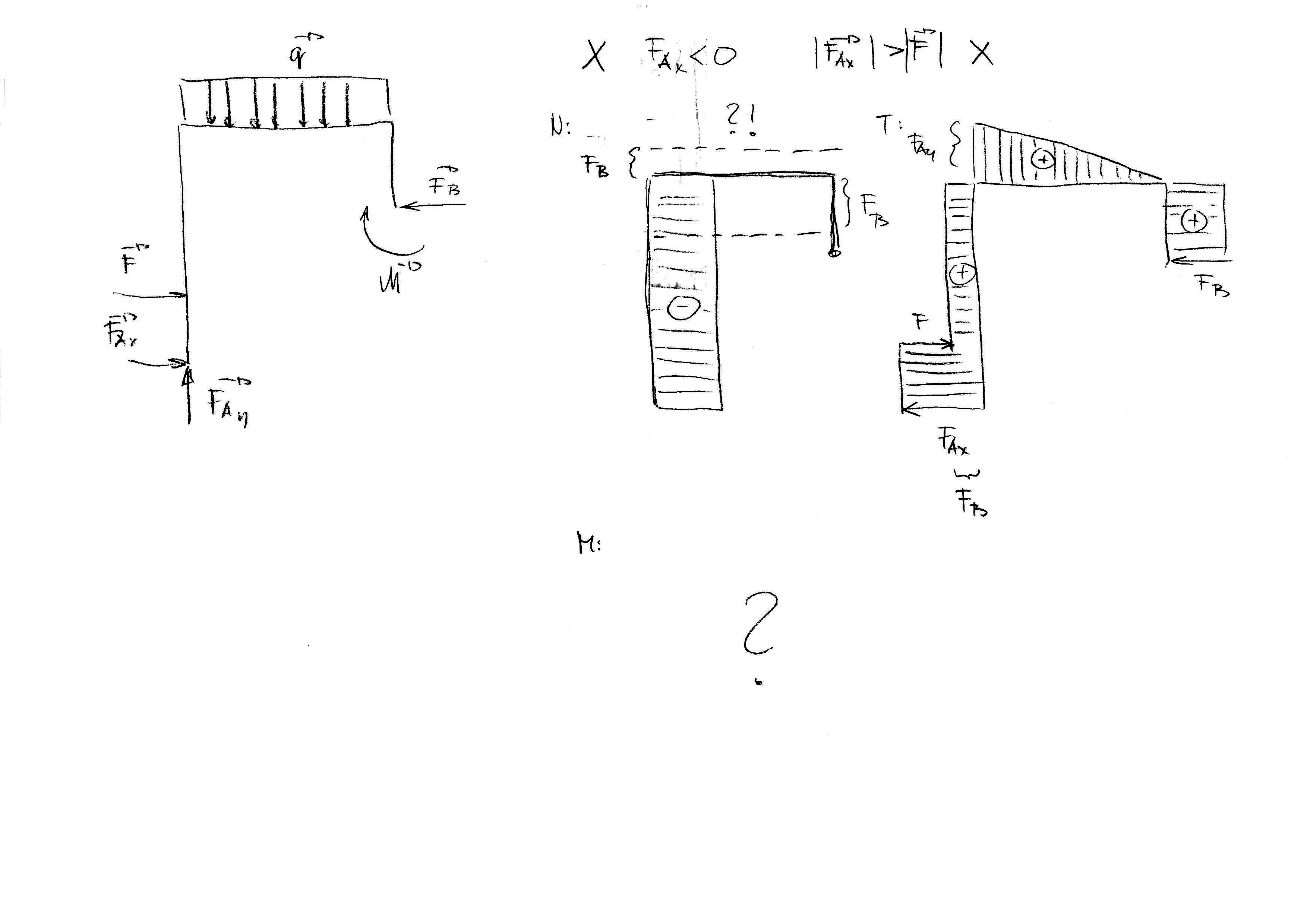
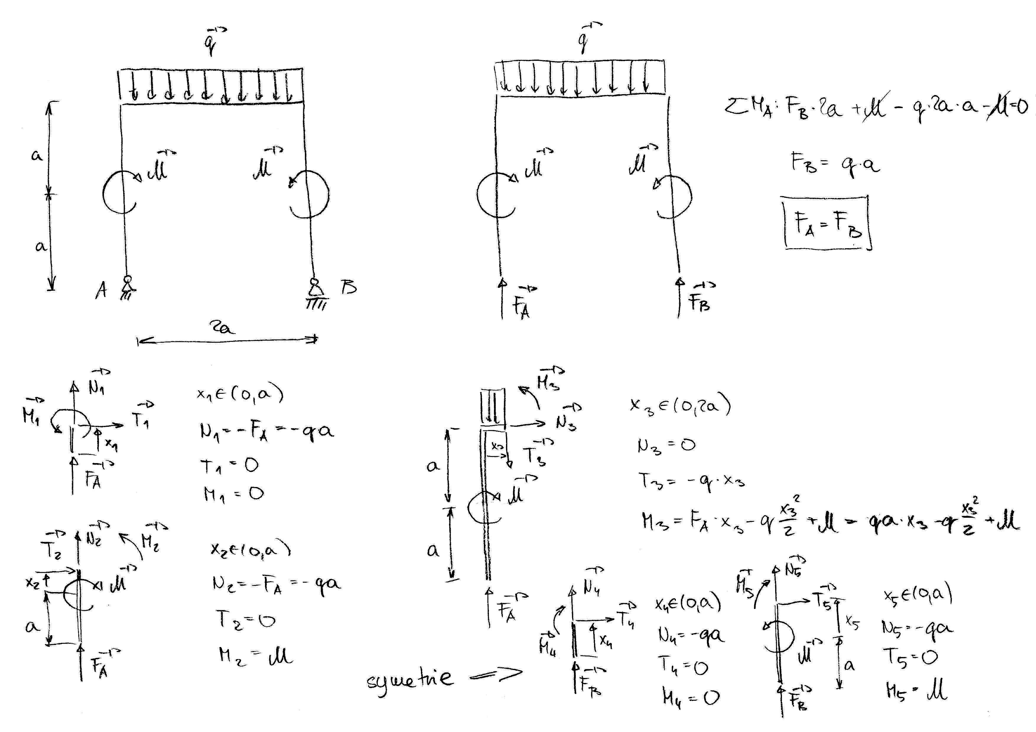
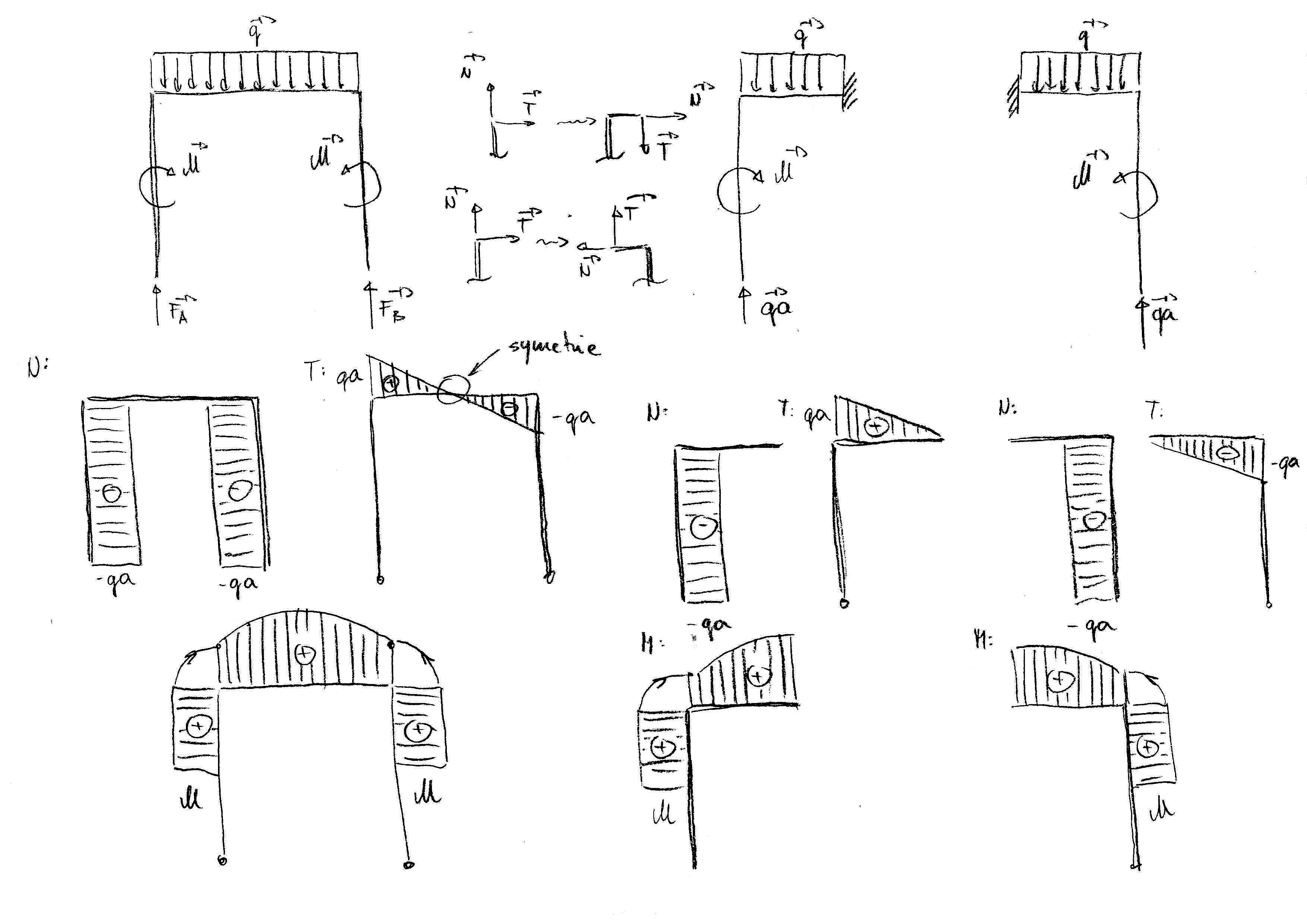
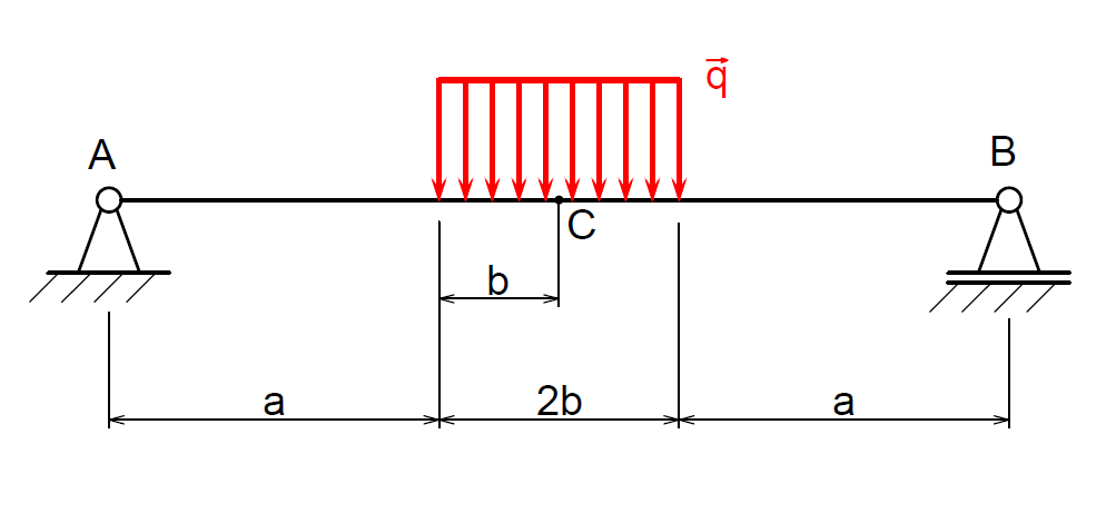
  • Cvičení 1: VVÚ přímého prutu.

    • Příklad v jazyce Julia - Př.1. Odpovídající soubor v Jupyteru lze stáhnout zde.

    • Další podklady:

  • Cvičení 2: VVÚ zalomených prutů.

    • Příklad v jazyce Python - Př.1. Odpovídající soubor v Jupyteru lze stáhnout zde. Obrázek lze stáhnout zde.

    • Příklad v jazyce Python - Př.2. Odpovídající soubor v Jupyteru lze stáhnout zde. Obrázek lze stáhnout zde.

    • Další podklady:

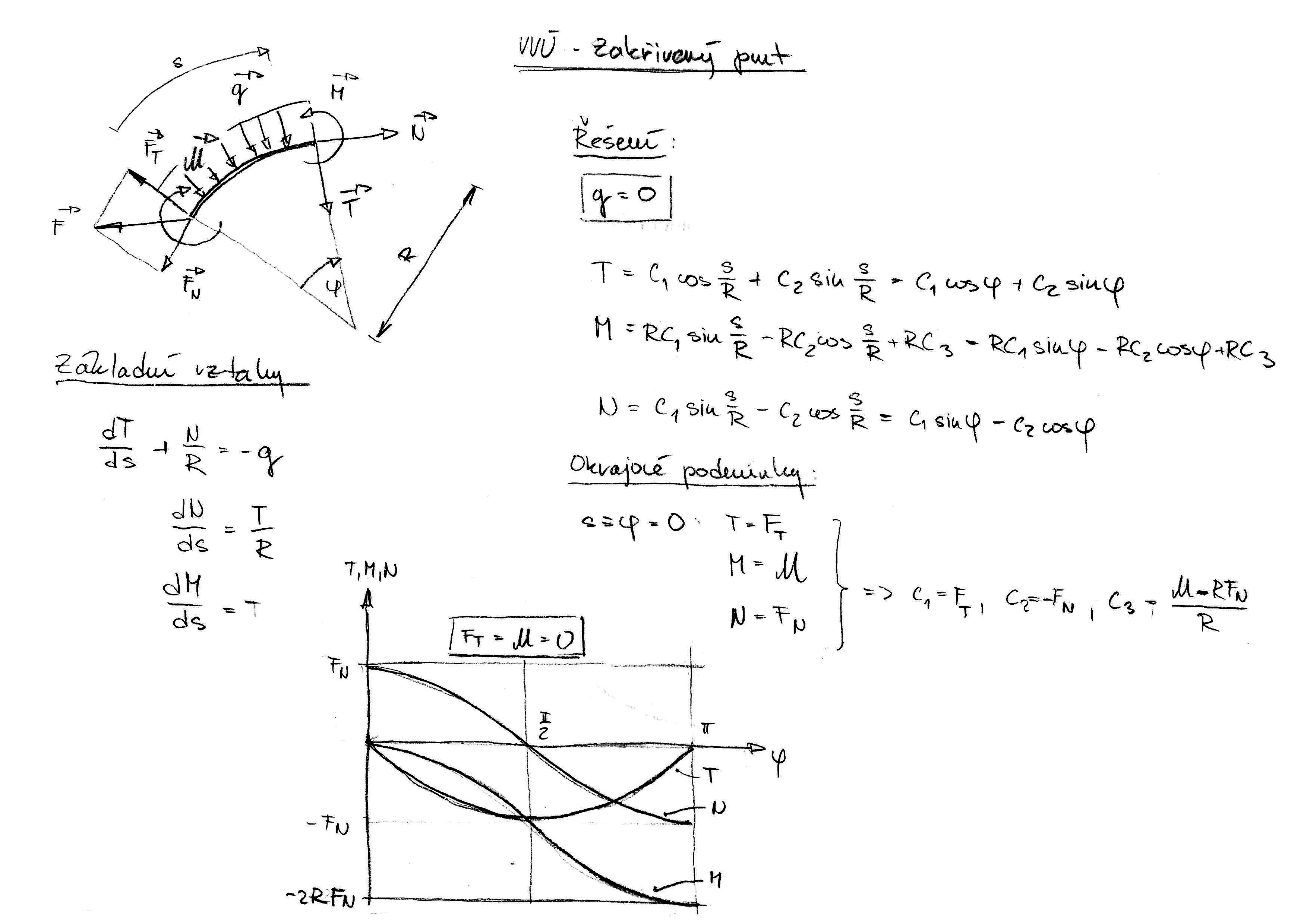
  • Cvičení 3: VVÚ zakřivených prutů.

    • Příklad v jazyce Python - Př.1. Odpovídající soubor v Jupyteru lze stáhnout zde.

    • Další podklady:

  • Cvičení 4: Průřezové charakteristiky.

    • Příklady v jazyce Python - Př.1-Př.3. Odpovídající soubor v Jupyteru lze stáhnout zde. Obrázky lze stáhnout zde, zde a zde.

    • Jednoduchá ukázka v jazyce Julia - Př.4 a odpovídající soubor v Jupyteru lze stáhnout zde.

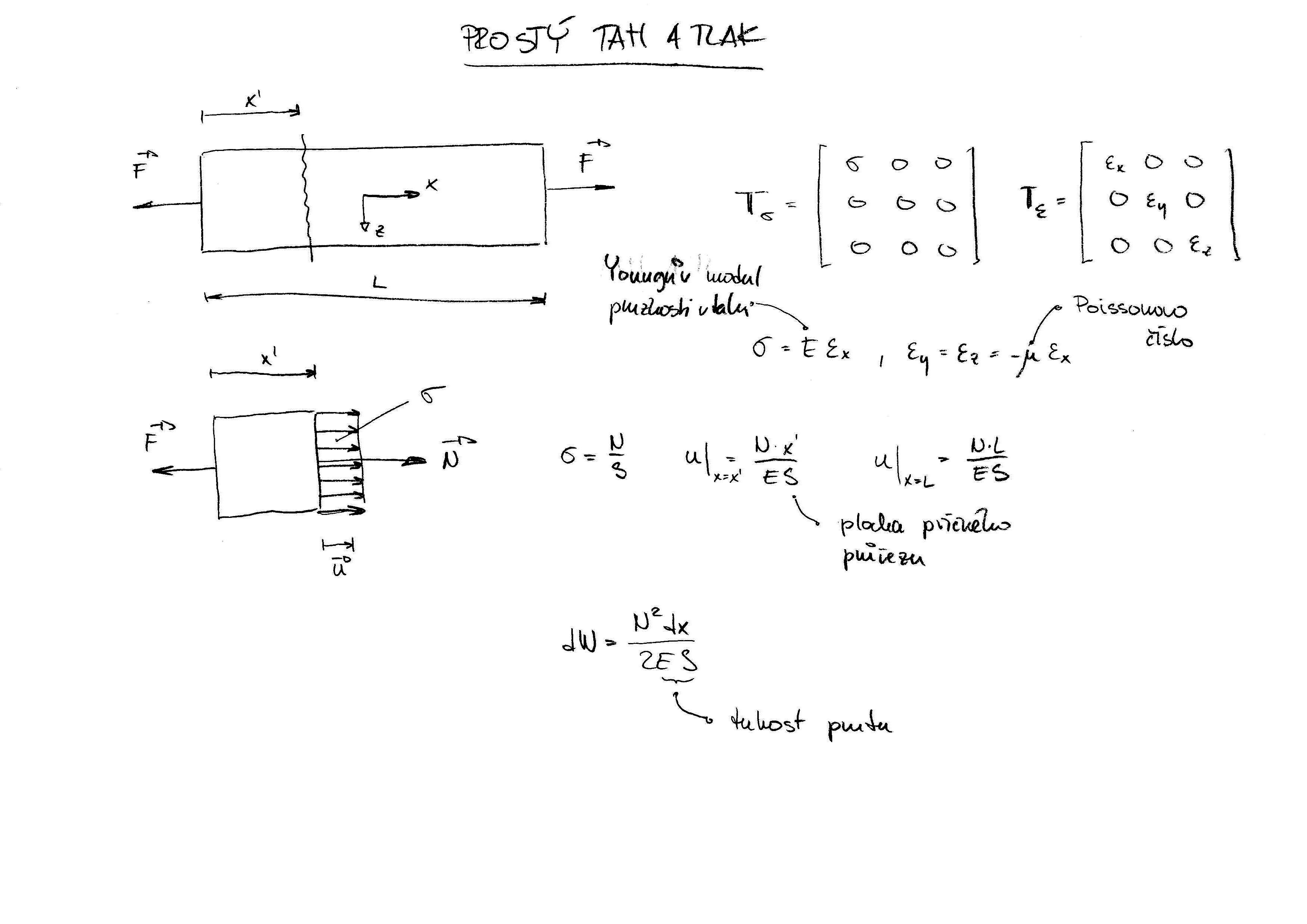
  • Cvičení 6: Prostý tah.

    • Příklad v jazyce Python - Př.1. Odpovídající soubor v Jupyteru lze stáhnout zde. Obrázky lze stáhnout zde a zde.

    • Příklad v jazyce Python - Př.2. Odpovídající soubor v Jupyteru lze stáhnout zde. Obrázky lze stáhnout zde, zde a zde.

    • Příklad v jazyce Python - Př.3. Odpovídající soubor v Jupyteru lze stáhnout zde. Obrázky lze stáhnout zde a zde.

    • Příklad v jazyce Python - Př.4. Odpovídající soubor v Jupyteru lze stáhnout zde. Obrázky lze stáhnout zde, zde a zde.

    • Příklad v jazyce Python - Př.5. Odpovídající soubor v Jupyteru lze stáhnout zde.

    • Příklad v jazyce Python - Př.6. Odpovídající soubor v Jupyteru lze stáhnout zde.

    • Numerické určení hodnot koncentrátoru napětí pomocí metody integrálních rovnic (BIE) je ukázáno zde.

    • Ručně řešený příklad Př.7 lze stáhnout zde.

    • Ručně řešený příklad Př.8 lze stáhnout zde.

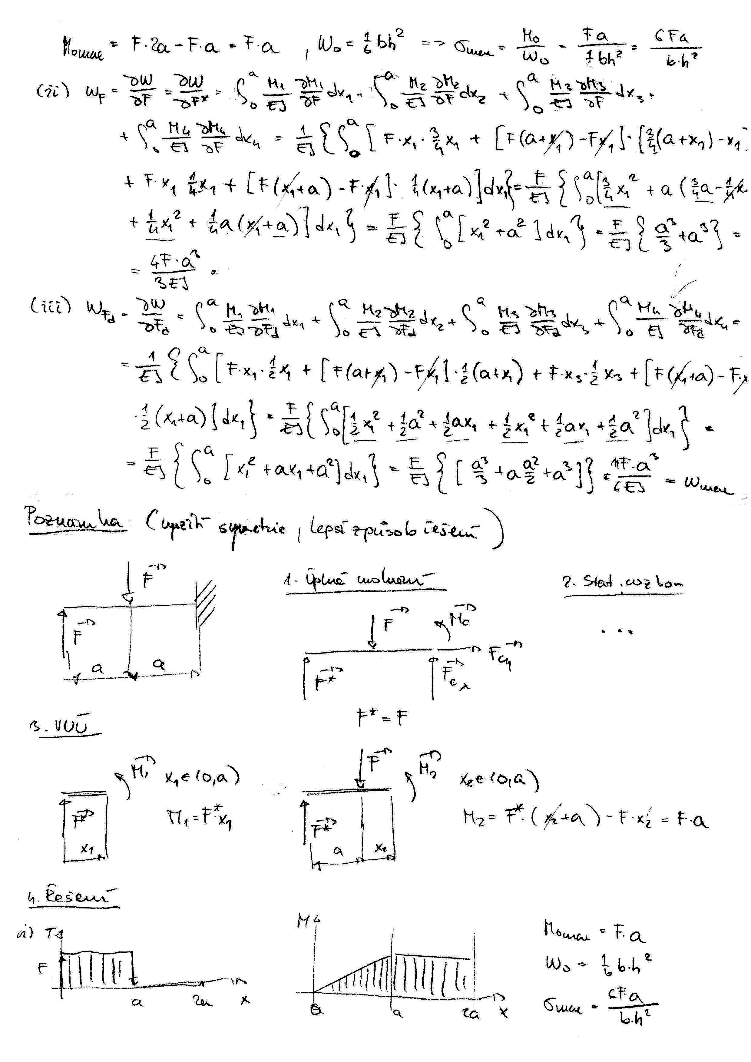
  • Cvičení 7: Ohyb přímých prutů.

    • Příklad v jazyce Python - Př.1. Odpovídající soubor v Jupyteru lze stáhnout zde. Obrázky lze stáhnout zde a zde.

    • Příklad v jazyce Python - Př.2. Odpovídající soubor v Jupyteru lze stáhnout zde.

    • Ručně řešený příklad Př.3 a Př.4 lze stáhnout zde.

    • Př.5 a Př.6 - Prostý ohyb staticky určitě uložených přímých prutů: mp4, mp4, jpg, jpg, jpg, jpg

  • Cvičení 8: Ohyb zalomených prutů.

    • Příklad v jazyce Python - Př.1. Odpovídající soubor v Jupyteru lze stáhnout zde. Obrázky lze stáhnout zde a zde.

    • Příklad v jazyce Python - Př.2. Odpovídající soubor v Jupyteru lze stáhnout zde. Obrázky lze stáhnout zde, zde a zde.

    • Příklad v jazyce Python - Př.3. Odpovídající soubor v Jupyteru lze stáhnout zde. Obrázky lze stáhnout zde a zde.

    • Př.4, Př.5 a Př.6 - Prostý ohyb staticky neurčitě uložených zalomených prutů: mp4, jpg, jpg, jpg, jpg, jpg, jpg

  • Cvičení 9: Ohyb zakřivených prutů.

    • Příklad v jazyce Python - Př.1. Odpovídající soubor v Jupyteru lze stáhnout zde. Obrázky lze stáhnout zde, zde a zde.

    • Příklad v jazyce Python - Př.2. Odpovídající soubor v Jupyteru lze stáhnout zde.

    • Př.3, Př.4 a Př.5 - Prostý ohyb soustavy přímého a zakřiveného prutu: mp4, jpg, jpg, jpg, jpg, jpg

    • Př.6, Př.7 a Př.8 - Prostý ohyb staticky neurčitě uložených zakřivených prutů: mp4, jpg, jpg, jpg, jpg, jpg, jpg

    • Př.9, Př.10 and Př.11 - Prostý ohyb staticky neurčitě uložených prutů: mp4, jpg, jpg, jpg, jpg, jpg, jpg, jpg, jpg, jpg, jpg

  • Cvičení 10: Ohyb - průhybová čára.

    • Příklad v jazyce Python - Př.1. Odpovídající soubor v Jupyteru lze stáhnout zde. Obrázek lze stáhnout zde.

    • Příklad v jazyce Python - Př.2. Odpovídající soubor v Jupyteru lze stáhnout zde.

  • Cvičení 12: Prostý krut.

    • Příklad v jazyce Python - Př.1. Odpovídající soubor v Jupyteru lze stáhnout zde. Obrázky lze stáhnout zde a zde.

    • Příklad v jazyce Python - Př.2. Odpovídající soubor v Jupyteru lze stáhnout zde.

    • Krut prizmatického prutu obdélníkového průřezu - ukázka numerického výpočtu krutu pomocí metody konečných prvků. Příklad v jazyce Python - Př.3. Odpovídající soubor v Jupyteru se může stáhnout zde a k němu nutné nutné datové soubory lze stáhnout zde, zde, zde, zde a zde.

    • Ručně řešené příklady lze stáhnout zde.

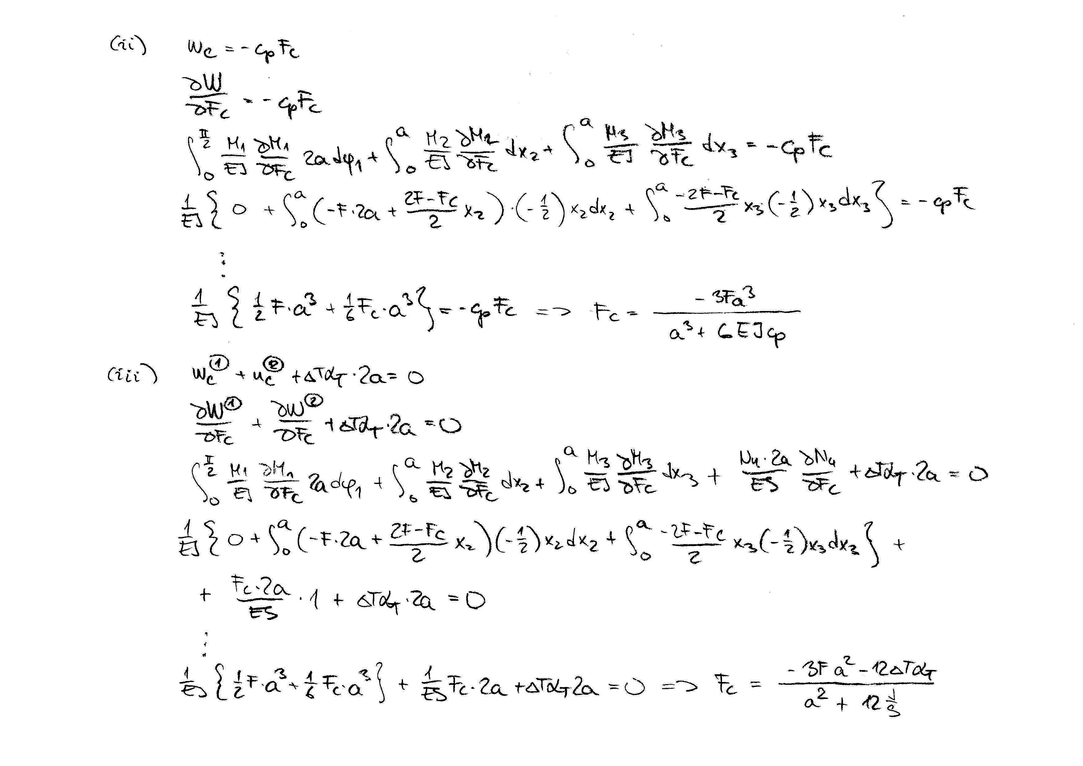
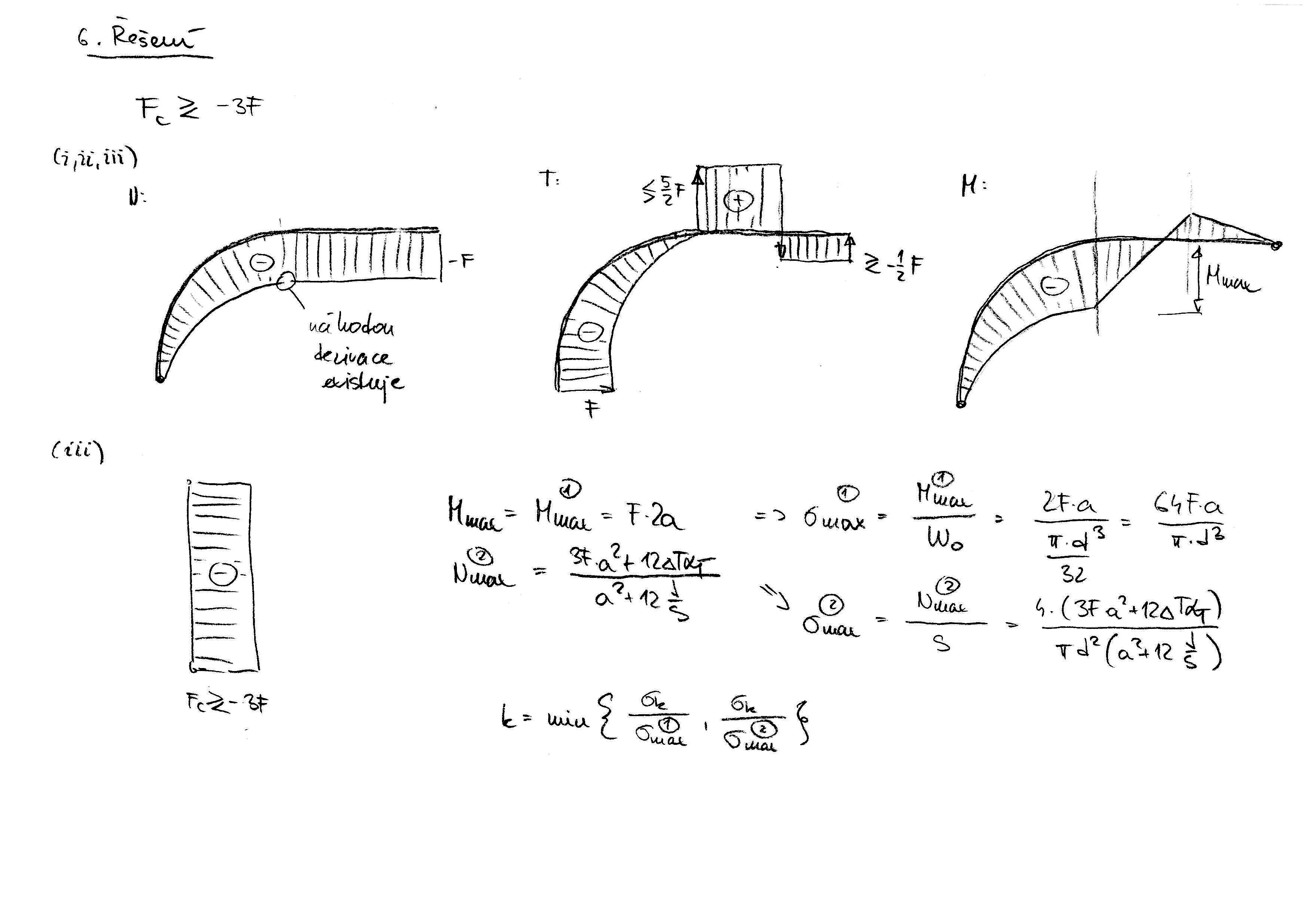
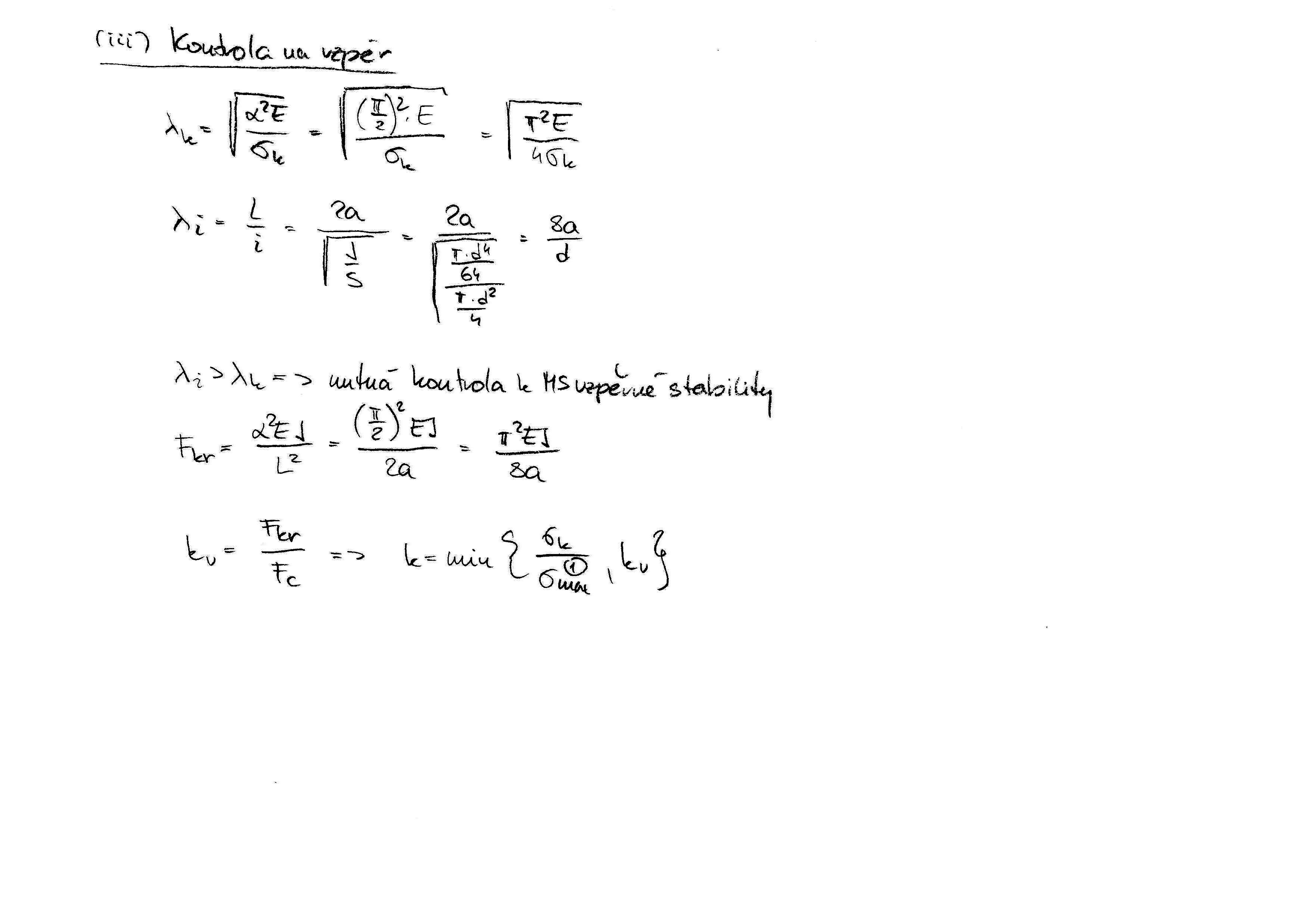
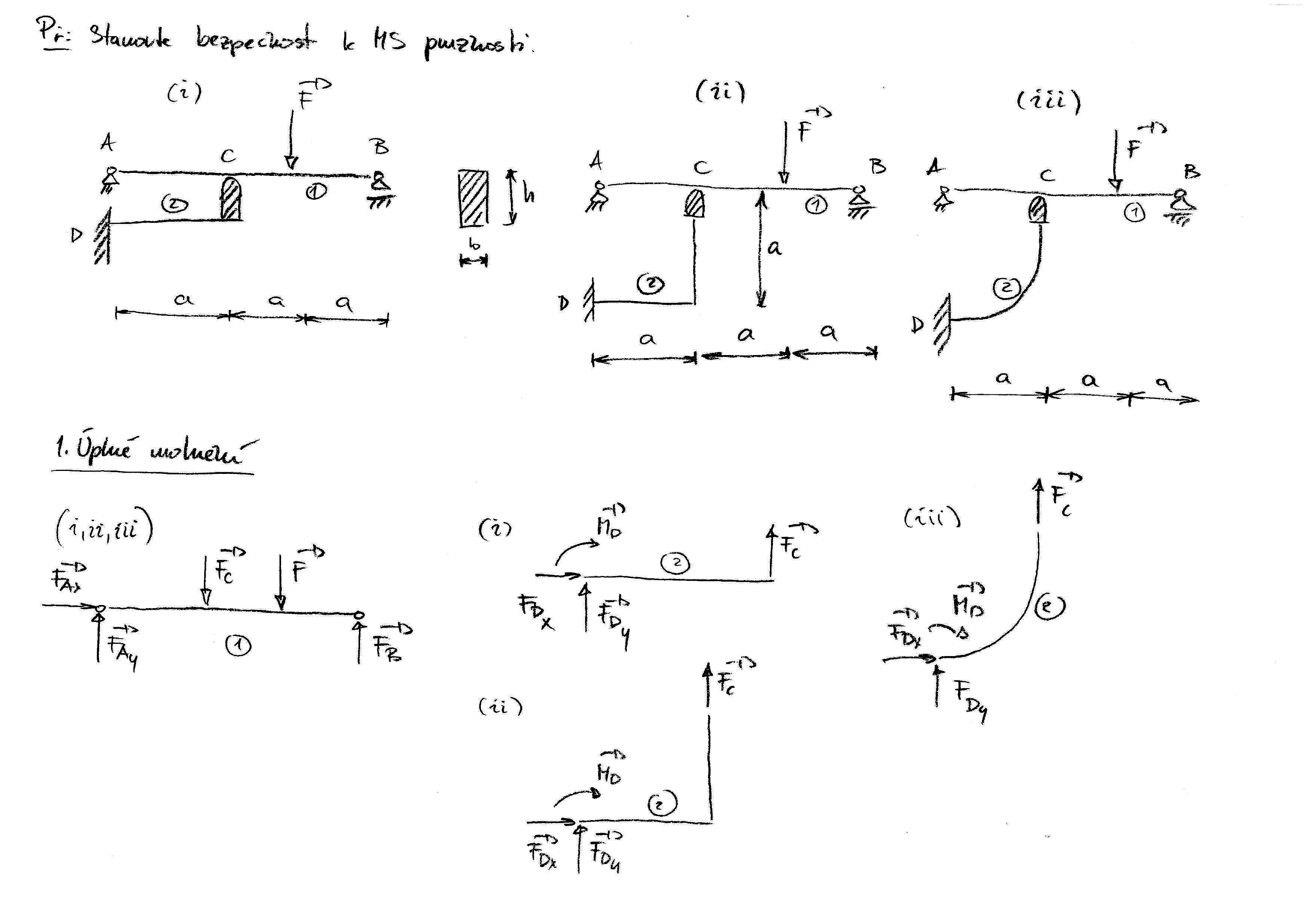
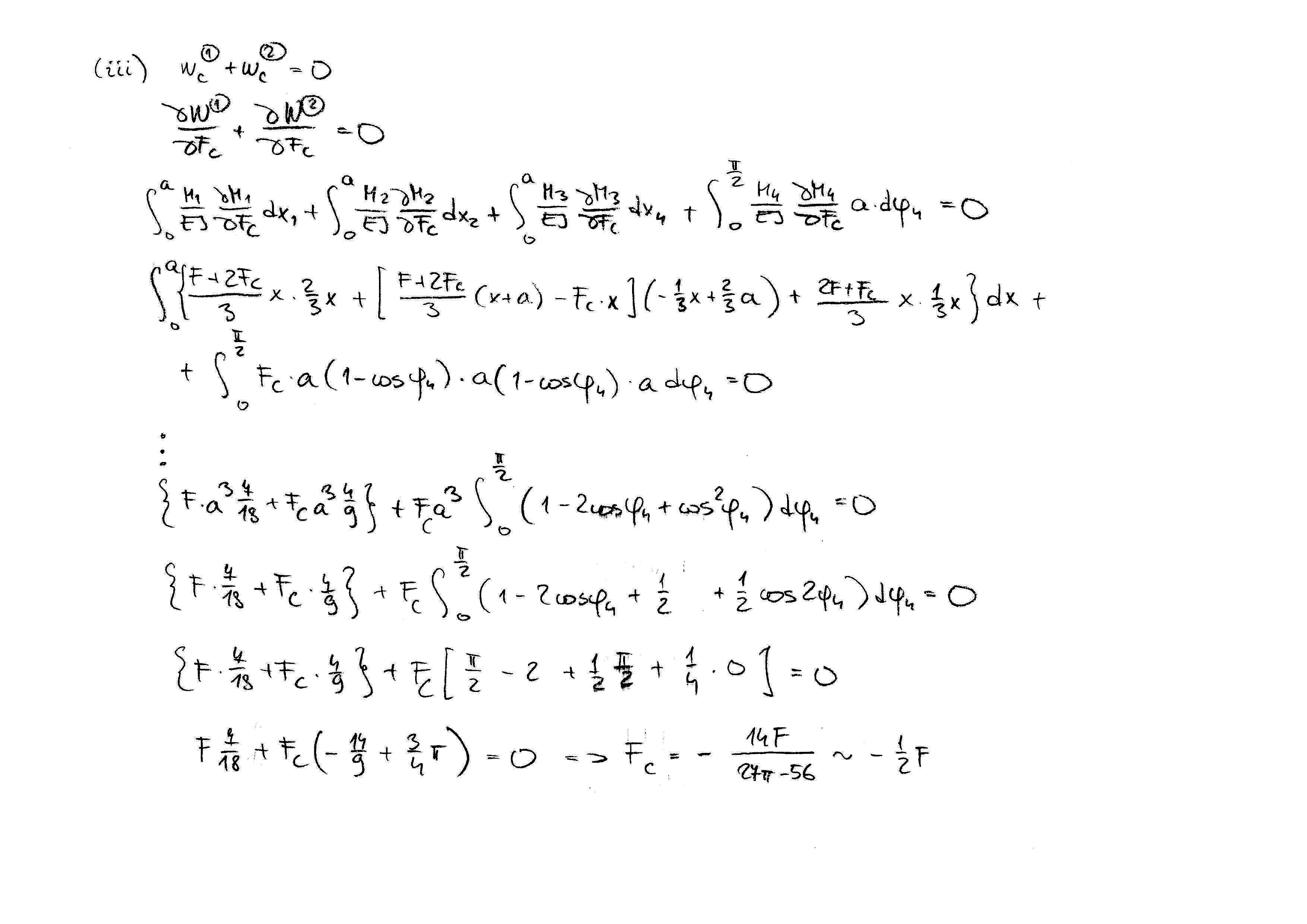
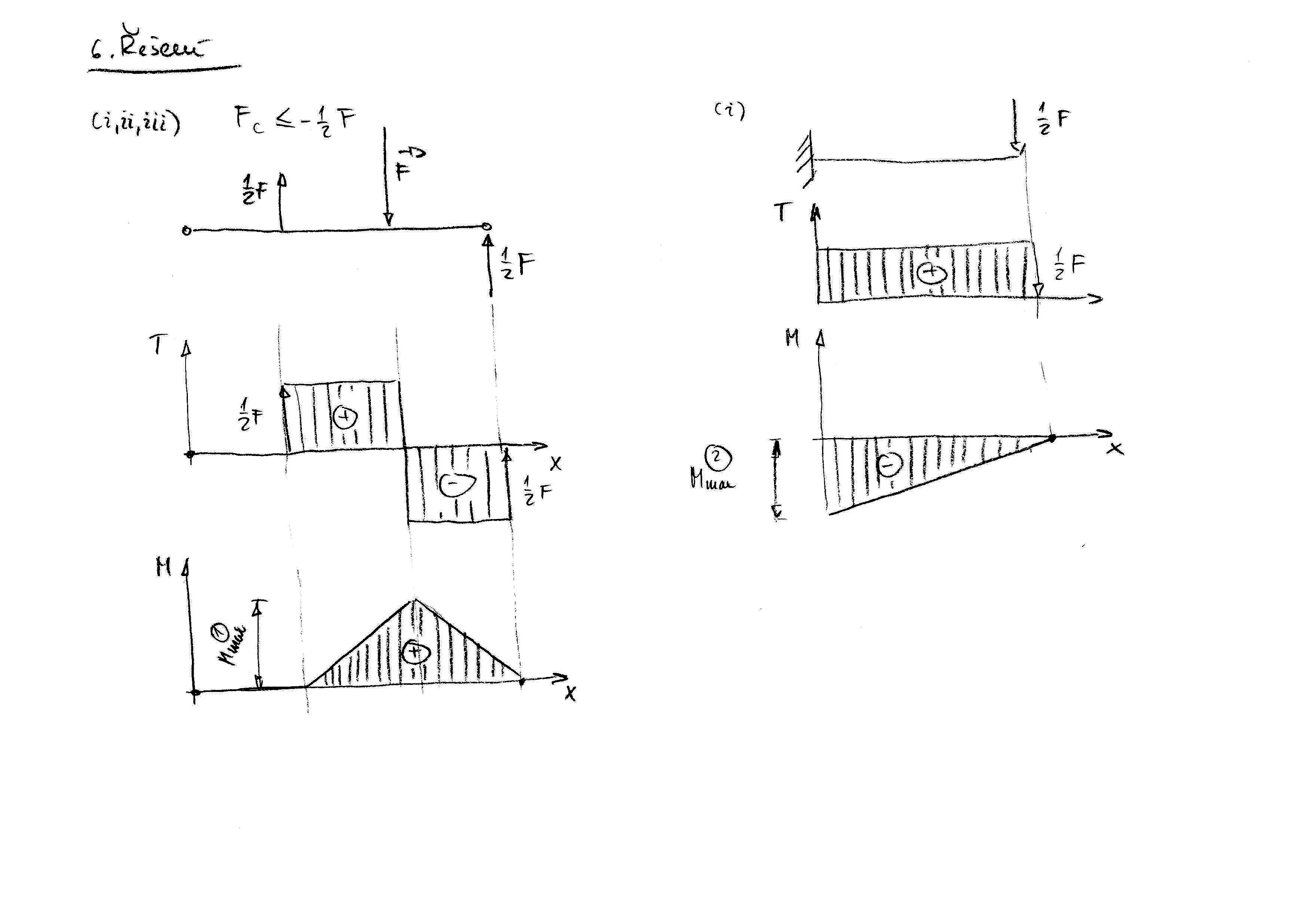
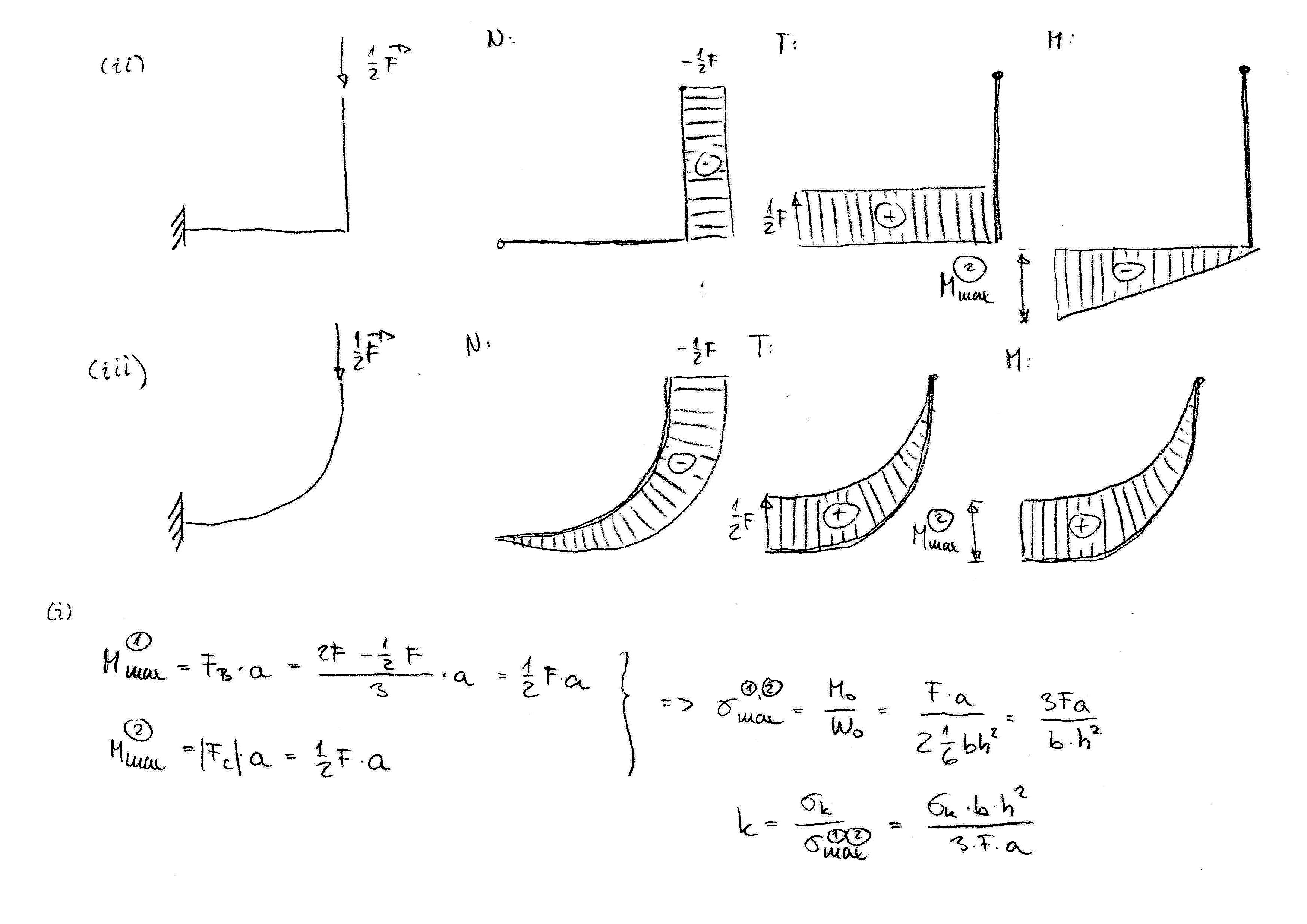
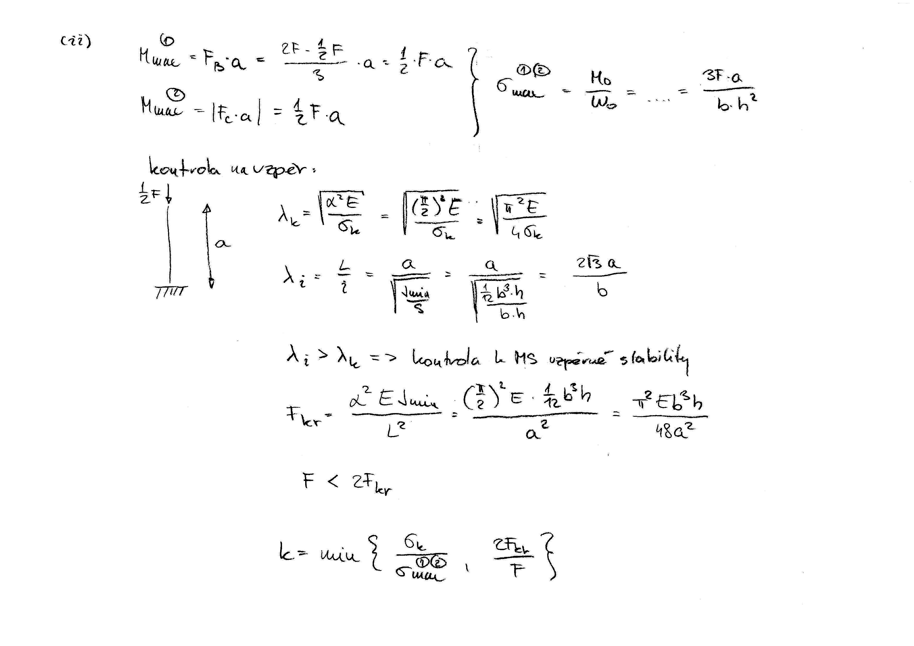
  • Cvičení 13: Kombinované namáhání a vzpěr.

    • Příklad v jazyce Python - Př.1. Odpovídající soubor v Jupyteru lze stáhnout zde. Obrázek se může stáhnout zde.

    • Ručně řešený příklad Př.2 lze stáhnout zde.

    • Ručně řešený příklad Př.3 lze stáhnout zde.

    • Ručně řešený příklad Př.4 lze stáhnout zde.

Pružnost a pevnost I-K

Požadavky ke zkoušce

Uvedené body jsou orientační, mohou být modifikovány.

Test (40 bodů) - vychází se z učebního textu, který lze stáhnout zde.

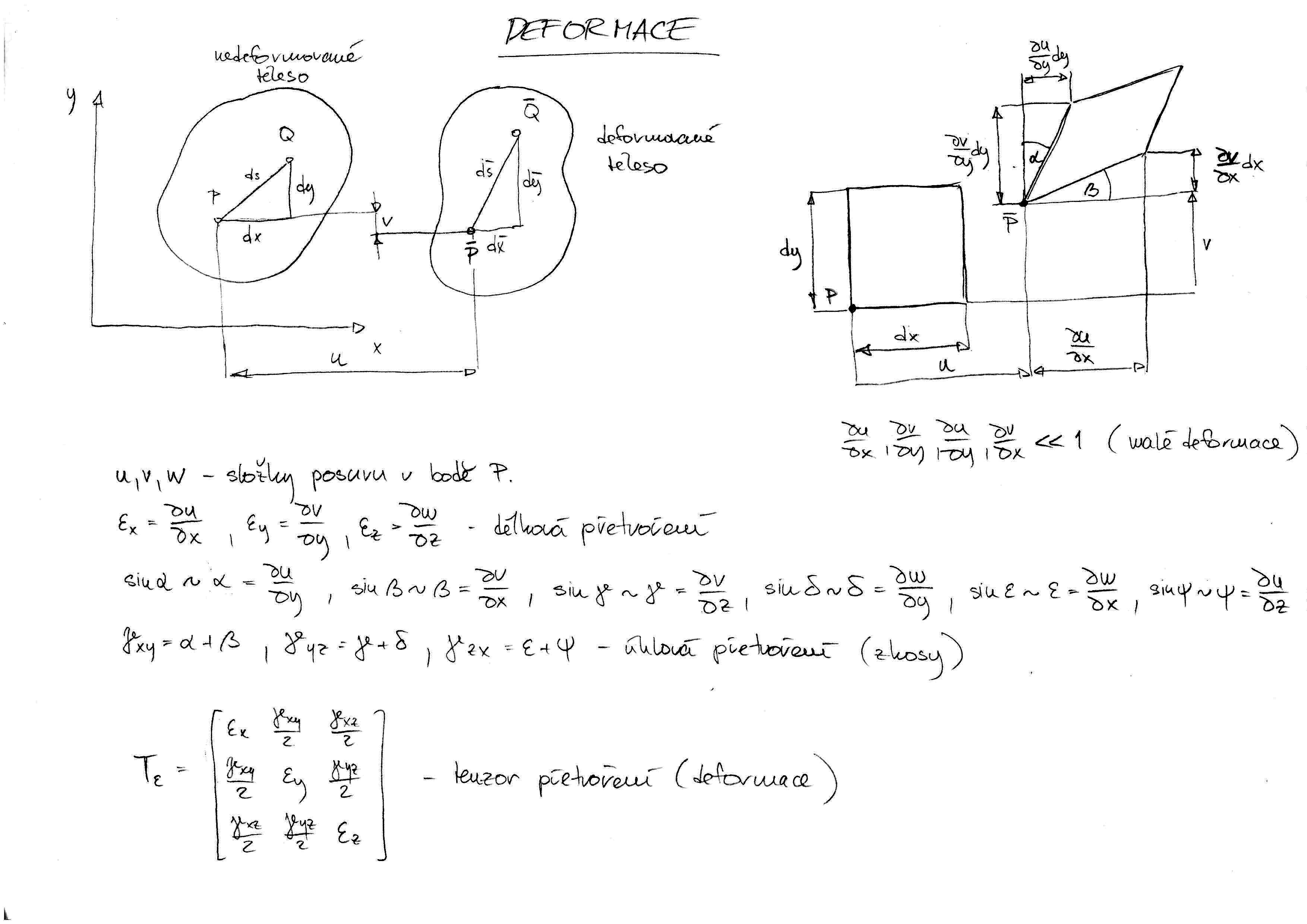
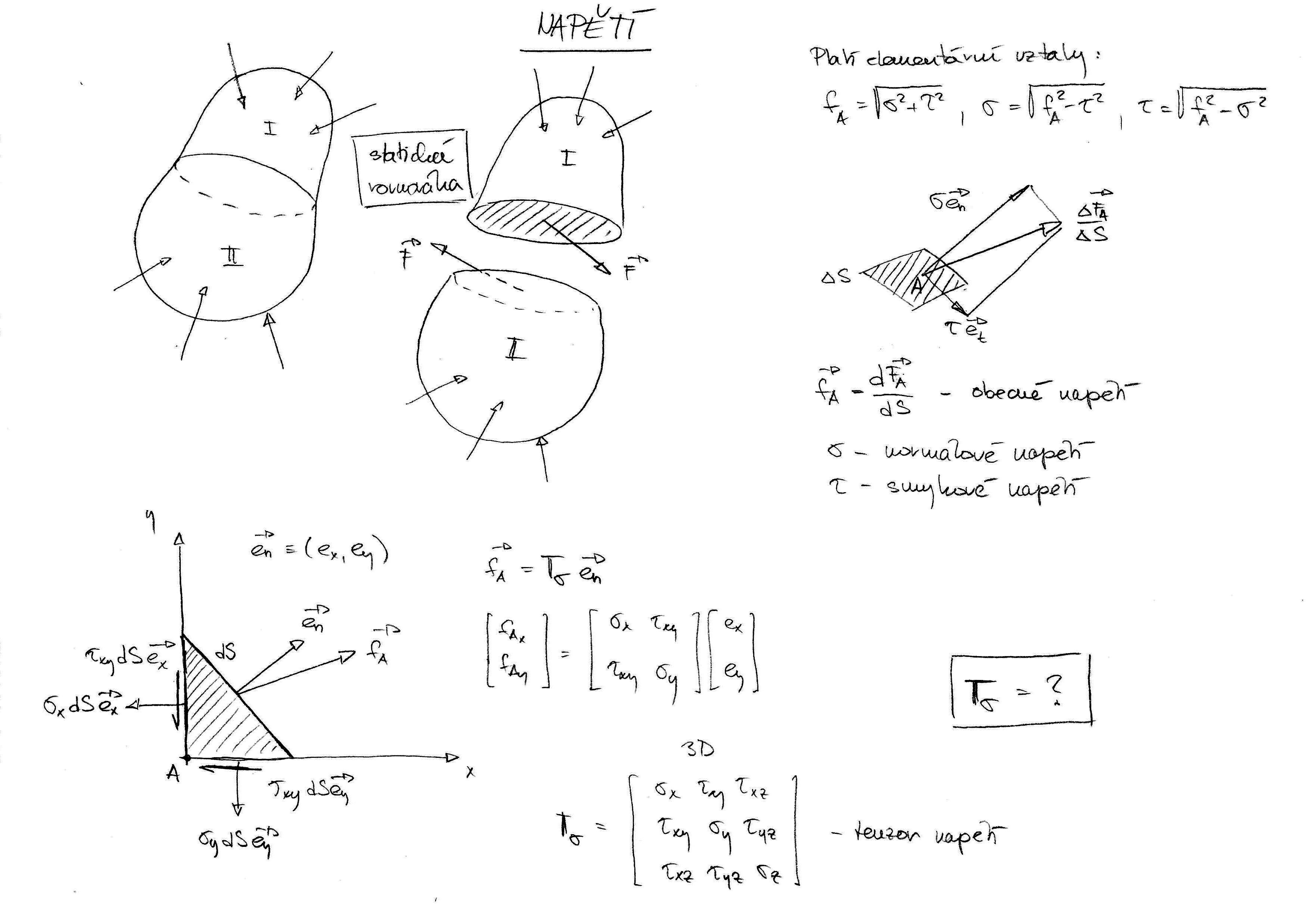
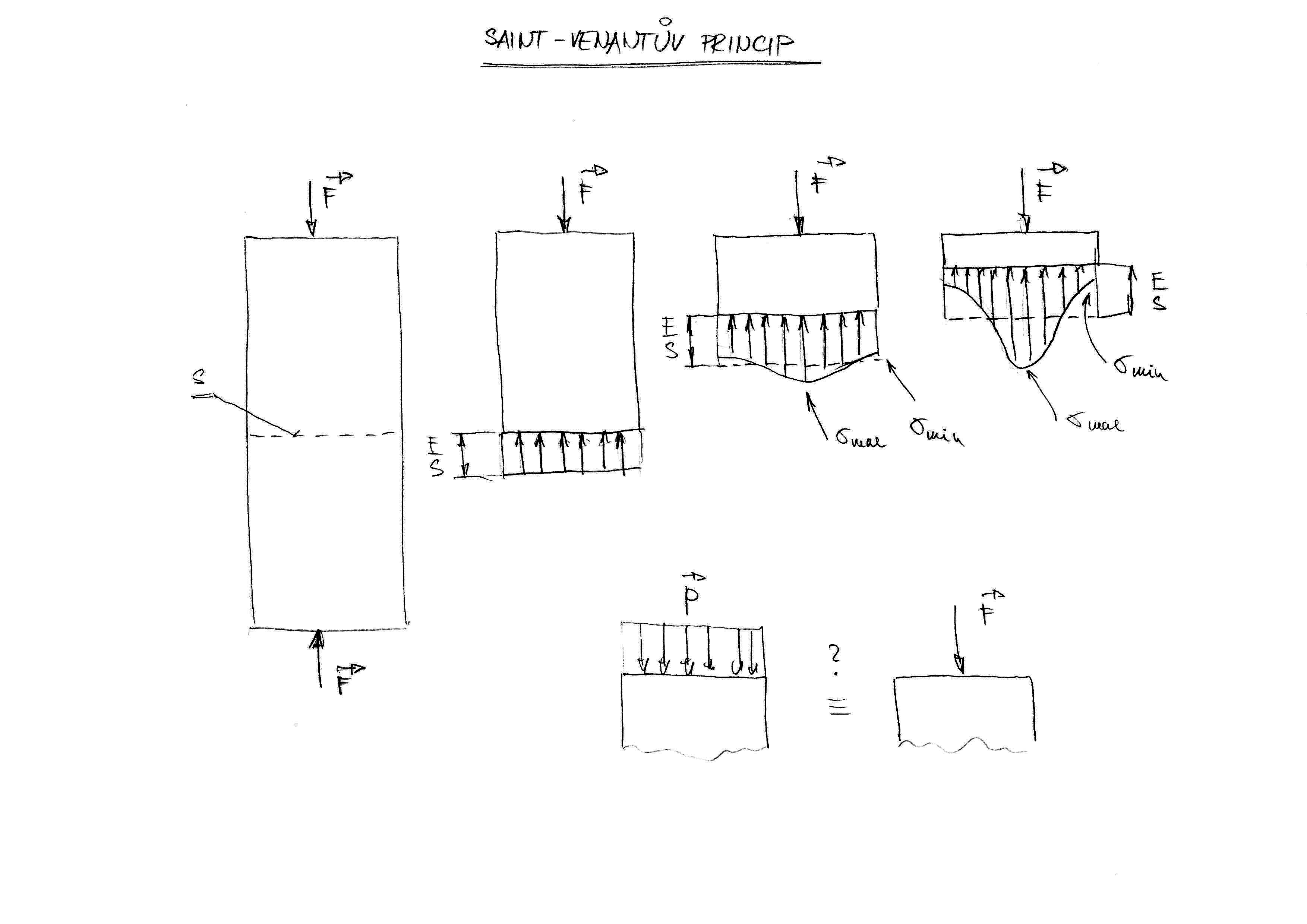
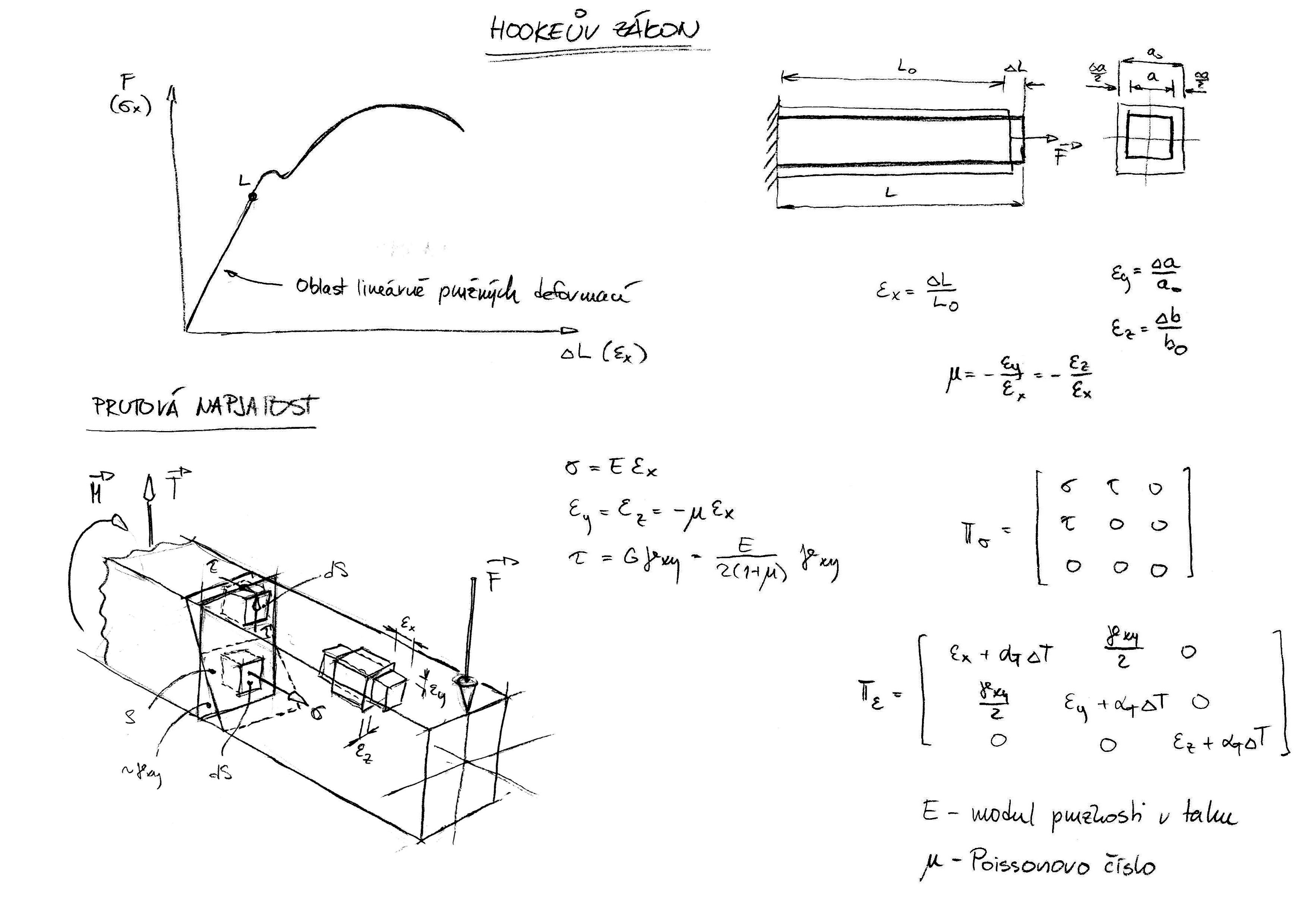
  • Základní pojmy (viz str. 3) - deformace tělesa (obrázky na str. 3, 5, vztahy 2.1, 2.2, 2.3), napjatost v bodě tělesa (vše str. 7-8), Saint-Venantův princip (str. 14).

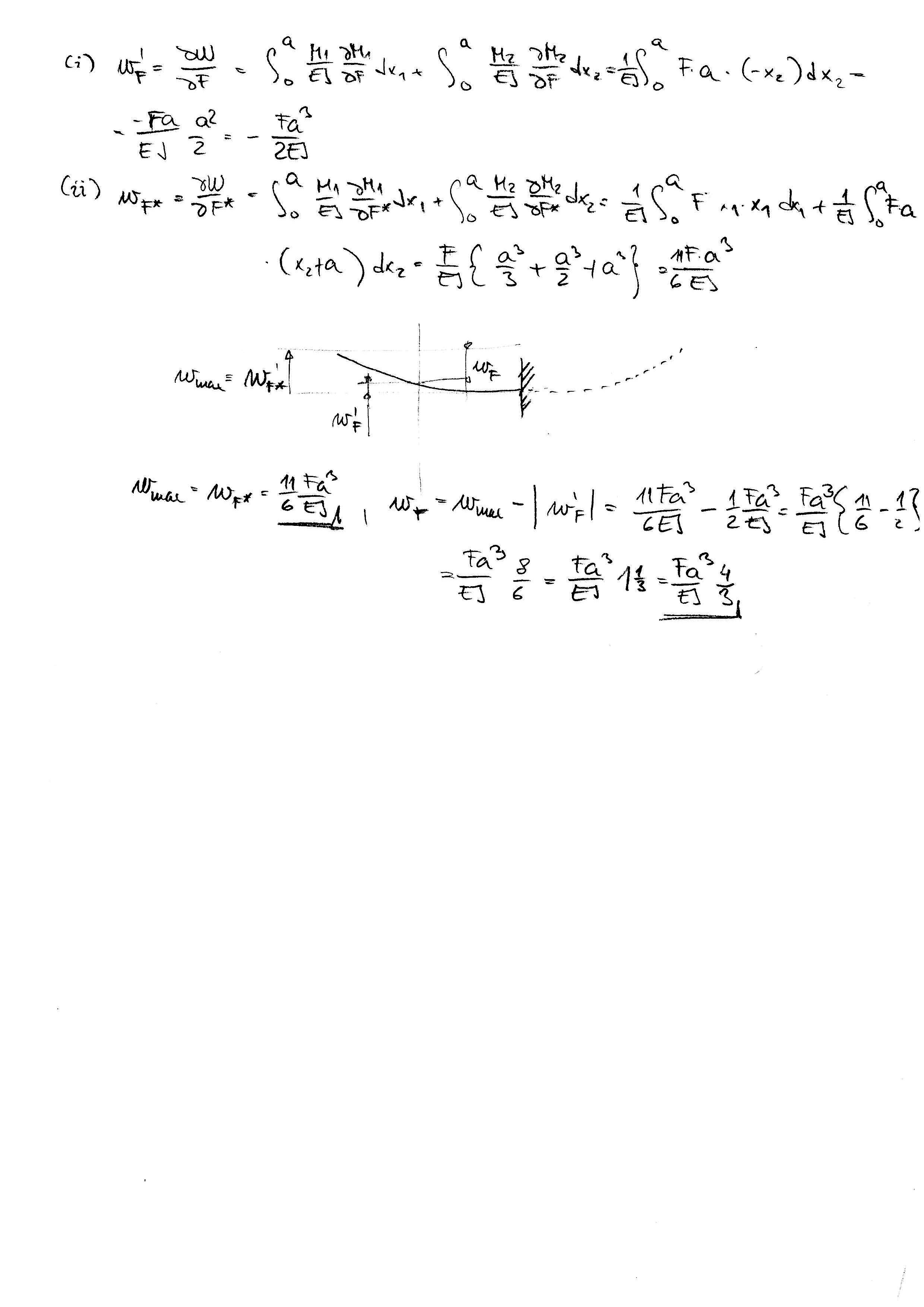
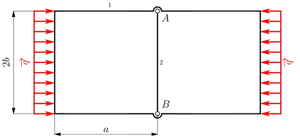
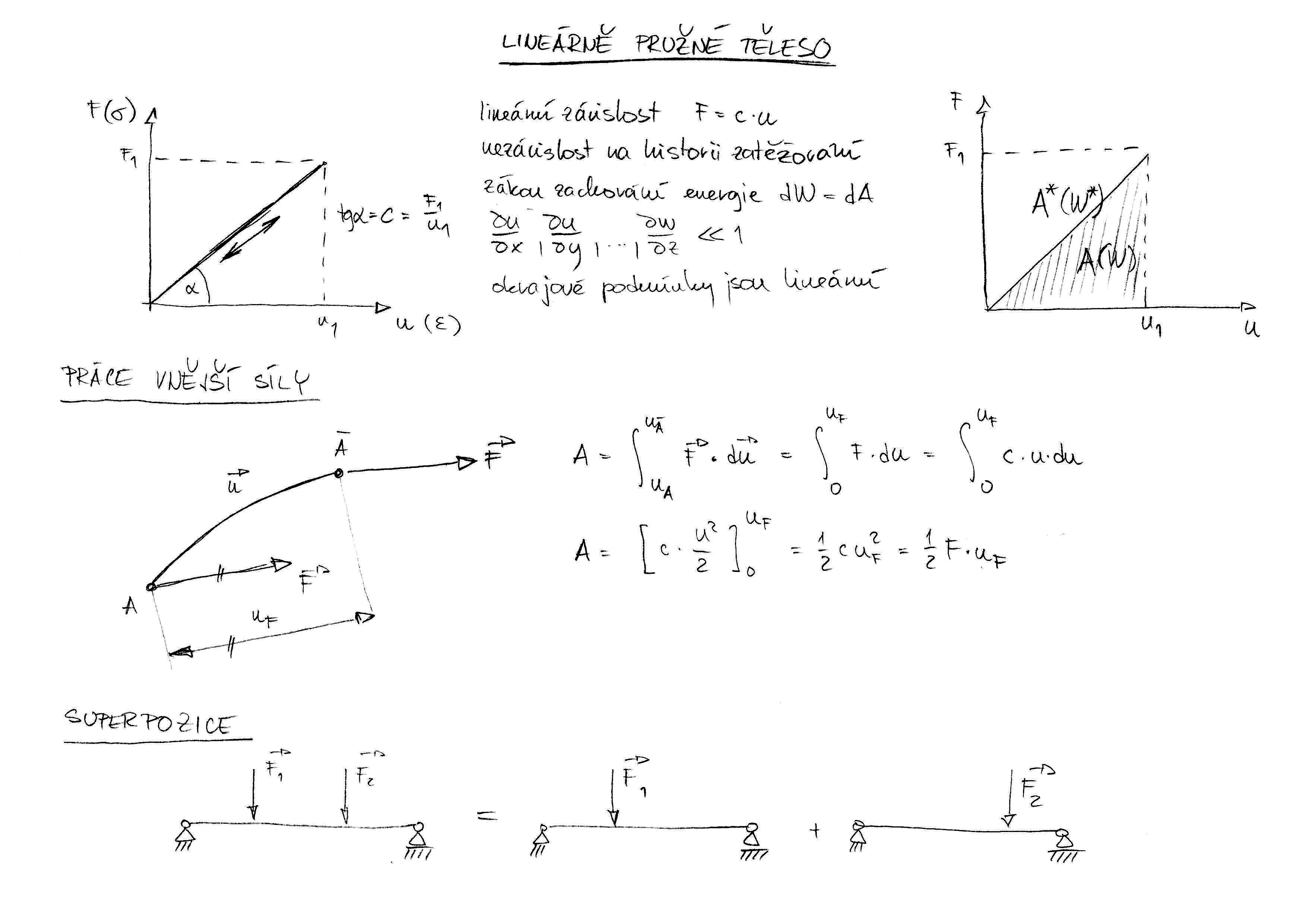
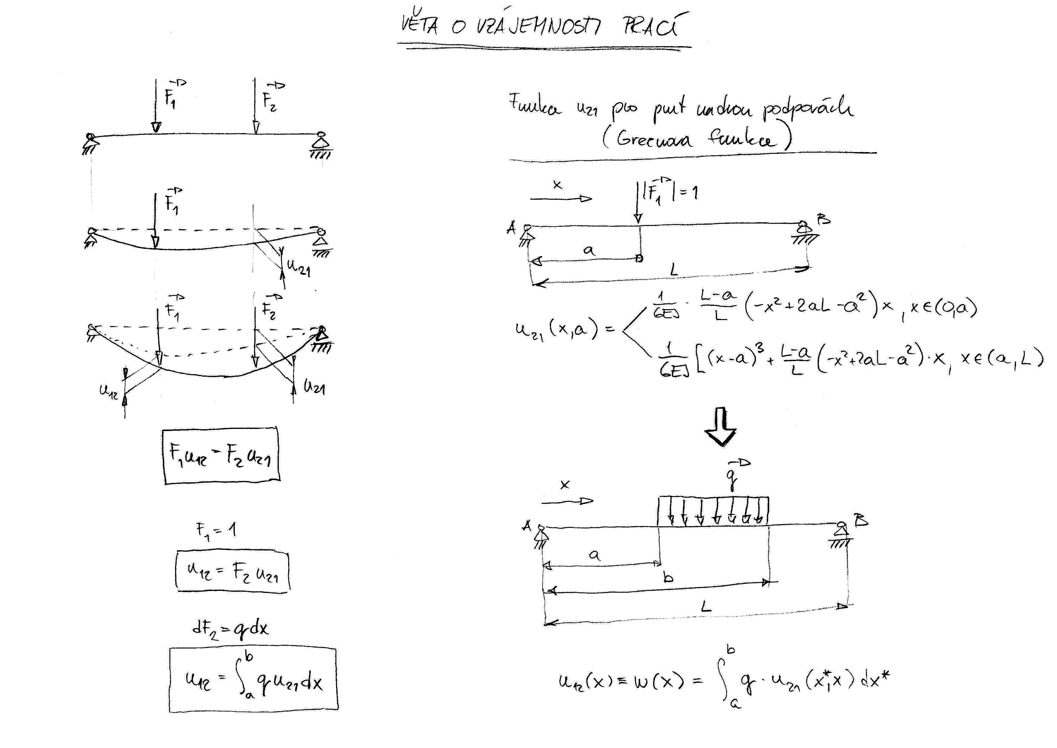
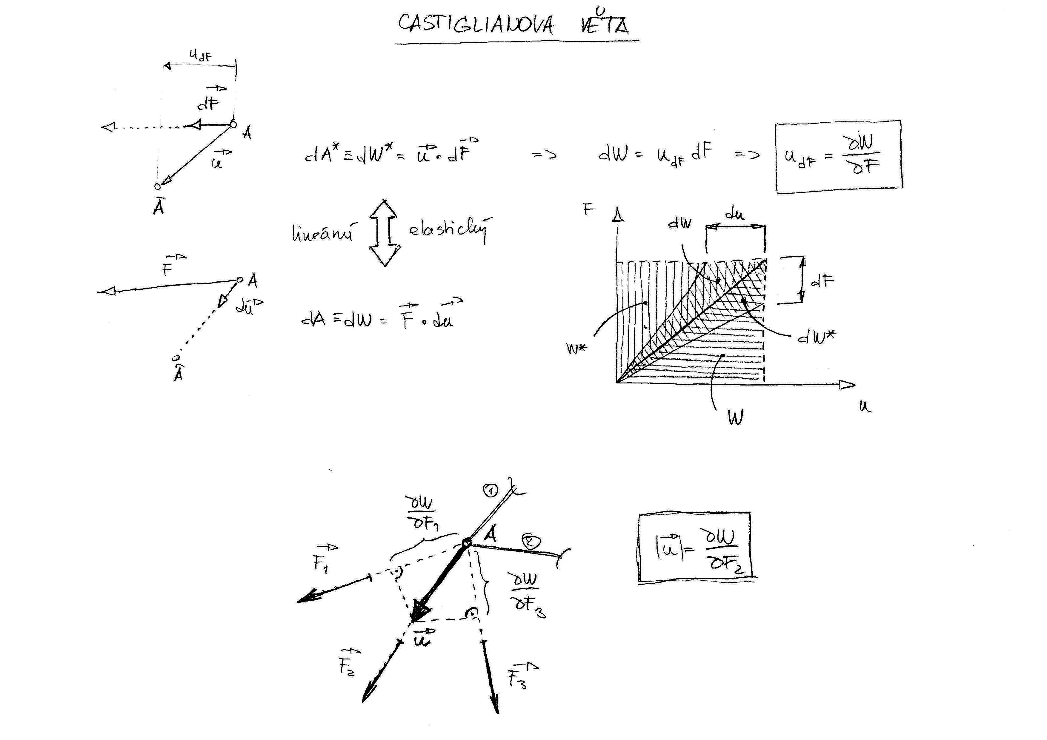
  • Obecné vlastnosti a obecné věty lineárně pružného tělesa (viz str. 23) - obrázky, vztahy a pojmy ze str. 23-24, deformační práce osamělé síly, věta o superpozici (str.25), věta o vzájemnosti prací (str 27 - vztah 3.6, slovní formulace), deformační práce silové dvojice (str. 28), věta o deformační práci silové soustavy (str. 29).

  • Základní materiálové charakteristiky, tahová a tlaková zkouška (viz str. 35) - Poissonovo číslo (vztah 4.3, 4.5), Hookeův zákon (vztah 4.4). (Přestože v testu nebude vyžadován, doporučuji se seznámit s součinitelem \(\kappa\) (vztah 4.8)).

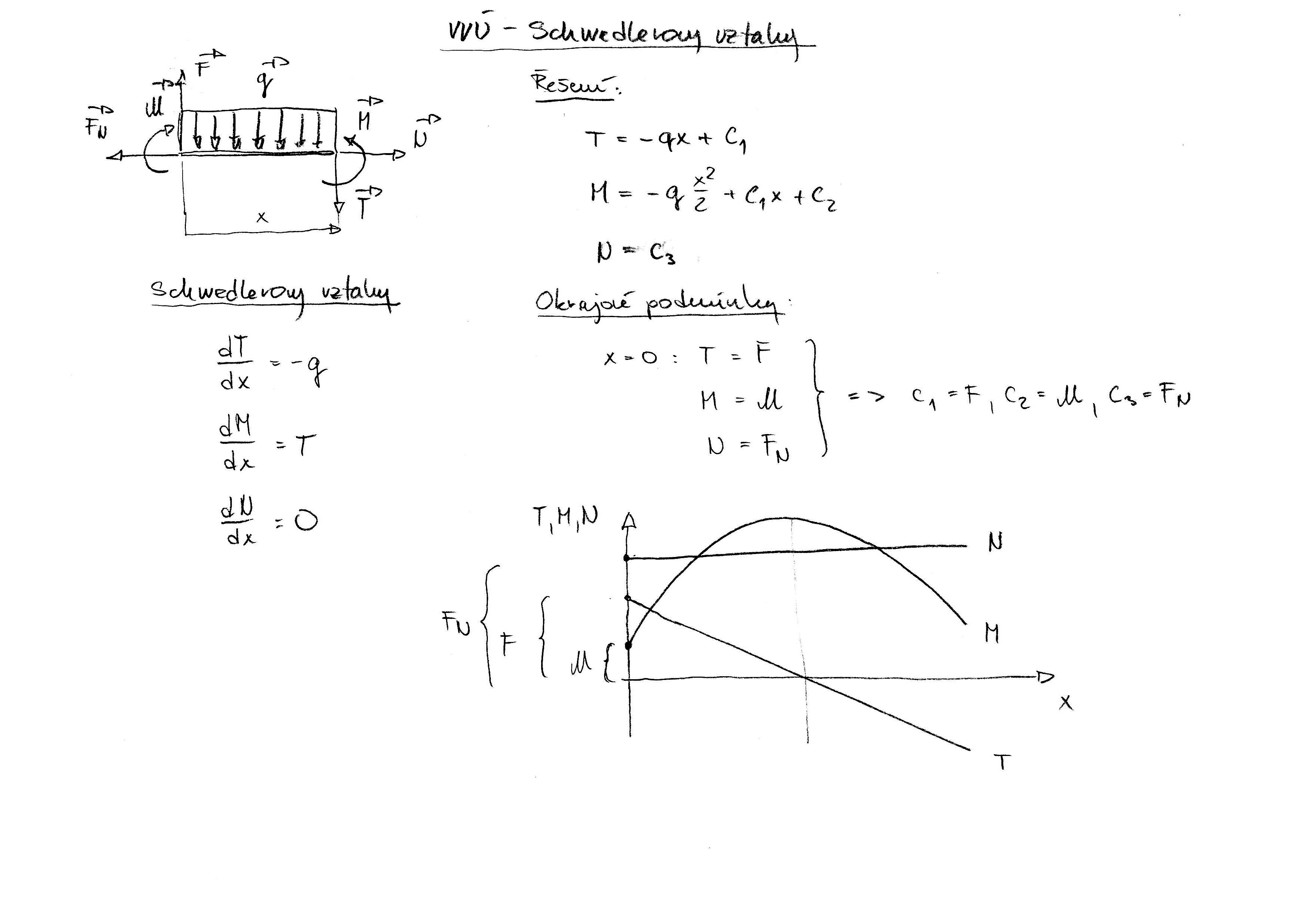
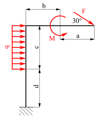
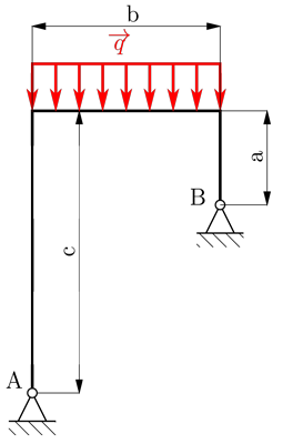
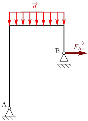
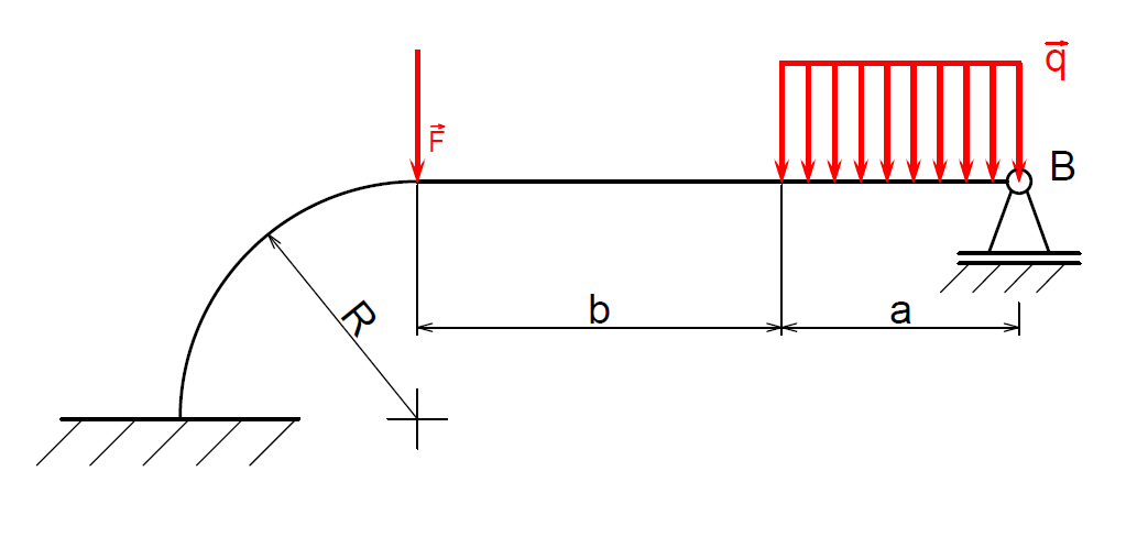
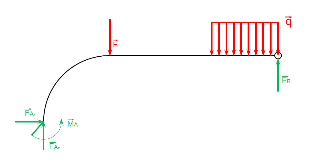
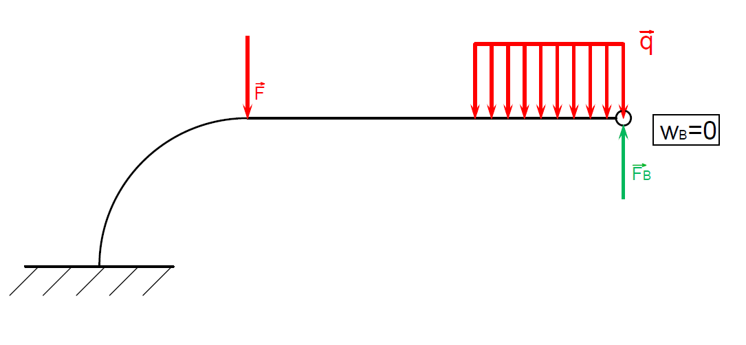
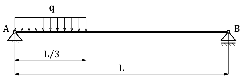
  • Prut v pružnosti a pevnosti (viz str. 44) - předpoklady geometrické (str. 44), předpoklady zatěžovací a vazbové (str. 45), předpoklady deformační (str. 45), předpoklady napjatostní (str. 46), Schwedlerovy vztahy (vztah 5.3, 5.4, 5.5, 5.6). Součástí testu bude i několik příkladů určení VVÚ graficky u přímých staticky určitě uložených prutů.

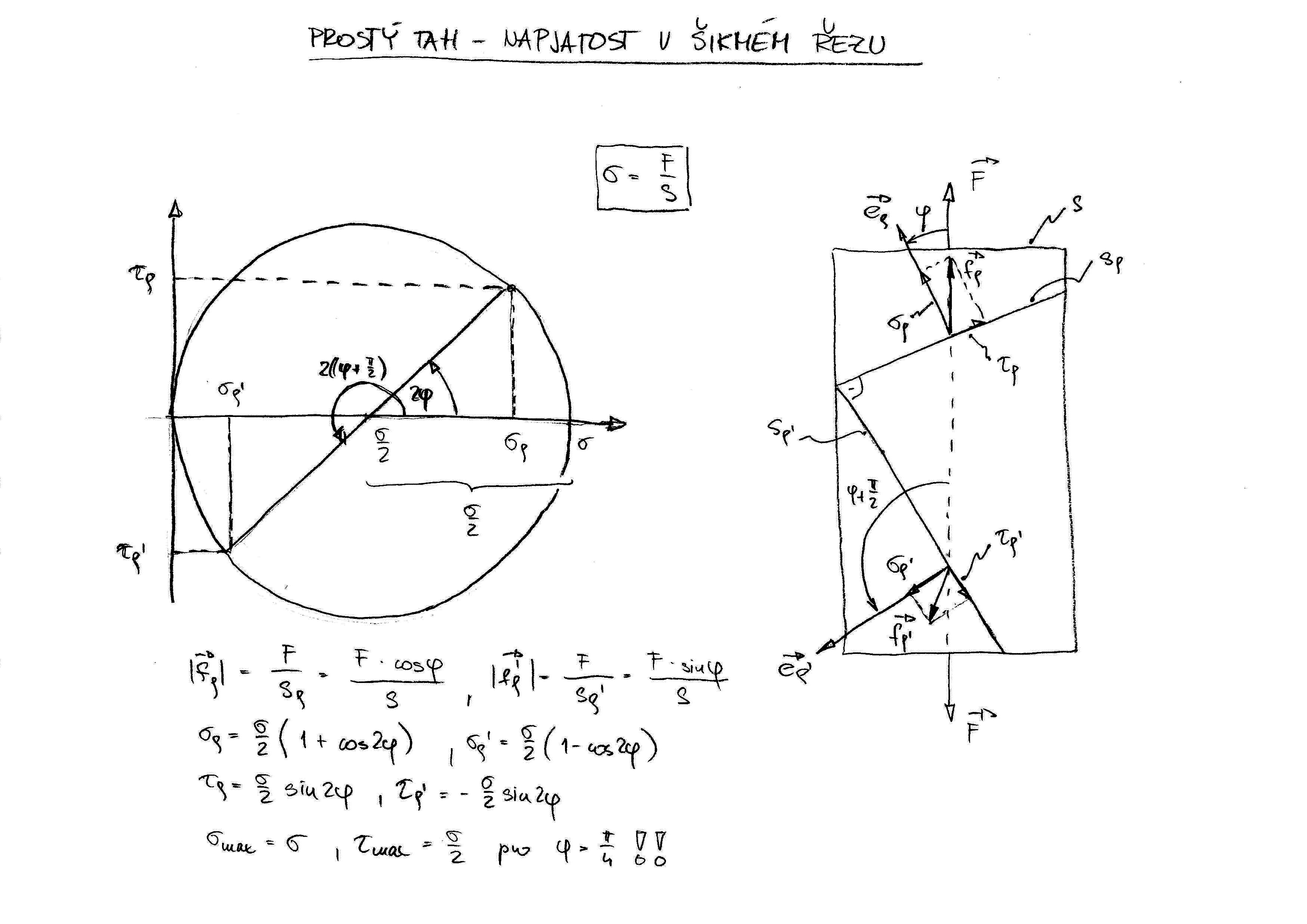
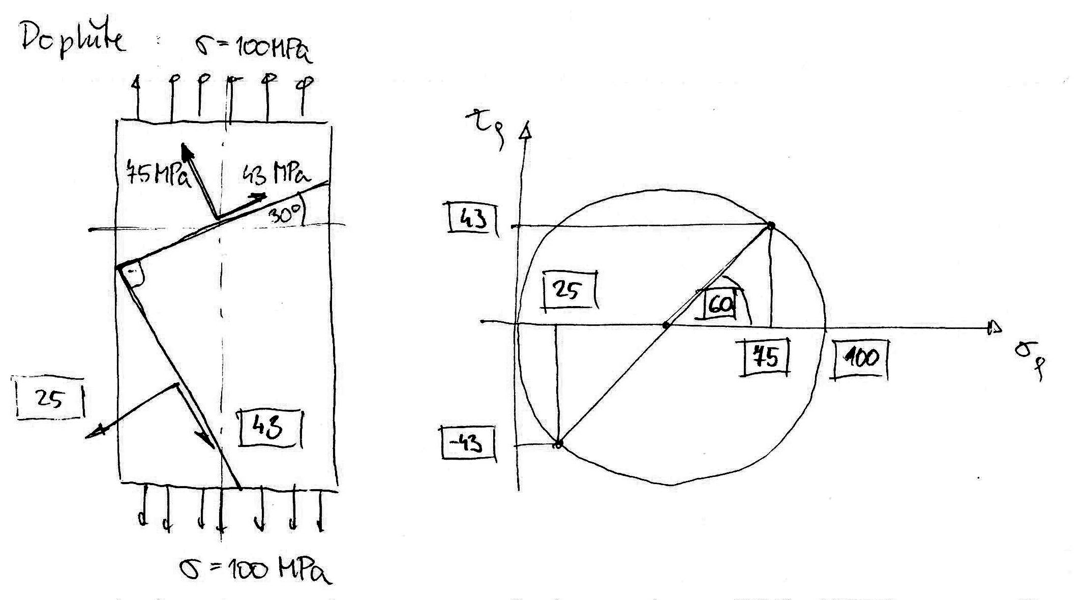
  • Namáhání na tah a tlak (viz str. 59) - definice (str. 59), vztahy pro napětí 6.8, 6.9, posunutí v bodě \(x\) (vztah 6.10), energie napjatosti (vztah 6.11, 6.12), napjatost v šikmém řezu (str. 63-66)}.

  • Namáhání na ohyb (viz str. 91) - definice (str. 91), vztahy pro napětí a deformaci 7.13 a 7.14, definice neutrální osy a kdy nastává shoda shoda polohy neutrální osy s nositelkou ohybového momentu (str. 96), nebezpečné místo průřezu (str. 97), vztah 7.22 pro energii napjatosti, rovnice průhybové čáry a sestavení okrajových podmínek a podmínek spojitosti a hladkosti průhybové čáry na konkrétním příkladu (str. 103-106), Žuravského vzorec (vztah 7.36), hodnota \(\tau_{max}\) pro obdélníkový (kruhový) průřez, definice středu smyku (str. 122).

  • Namáhání na krut (viz str. 171) - natočení v místě \(x\) střednice prutu (vztah 8.6), napětí v bodě příčného průřezu (vztah 8.8), energie napjatosti (vztah 8.15).

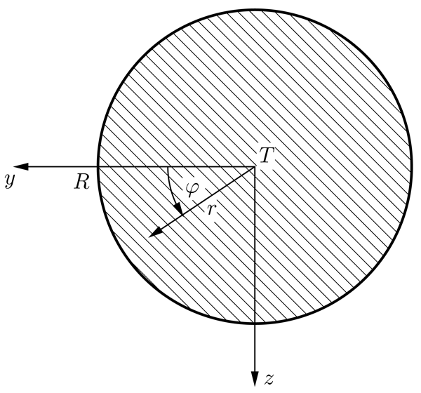
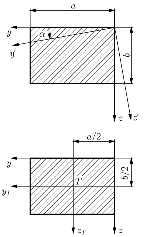
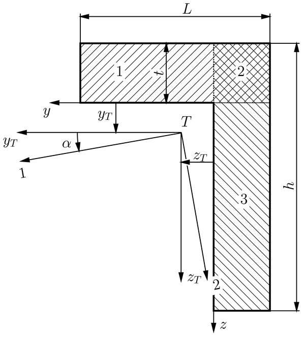
  • Průřezové charakteristiky (nebudou vyžadovány u testu, viz příloha A, str. 256) - definice průřezových charakteristik (str. 257-258), základní vlastnosti kvadratických momentů (str. 259-260), Steinerovy věty (vztah 15, str. 262), tenzor kv. momentů plochy \(\boldsymbol{T}_J\) (vztah 20, str. 266), definice hlavního souřadnicového systému, definice hlavního centrálního souřadnicového systému, vztah pro vyjádření úhlu \(\varphi_I\) (vztah 21, str. 266), nakreslení Möhrovy kružnice pro \(\boldsymbol{T}_J\) pro konkrétní hodnoty \(J_y\), \(J_z\) a \(J_{yz}\) (str. 268), doporučuji si projít příklady na str. 270-280.

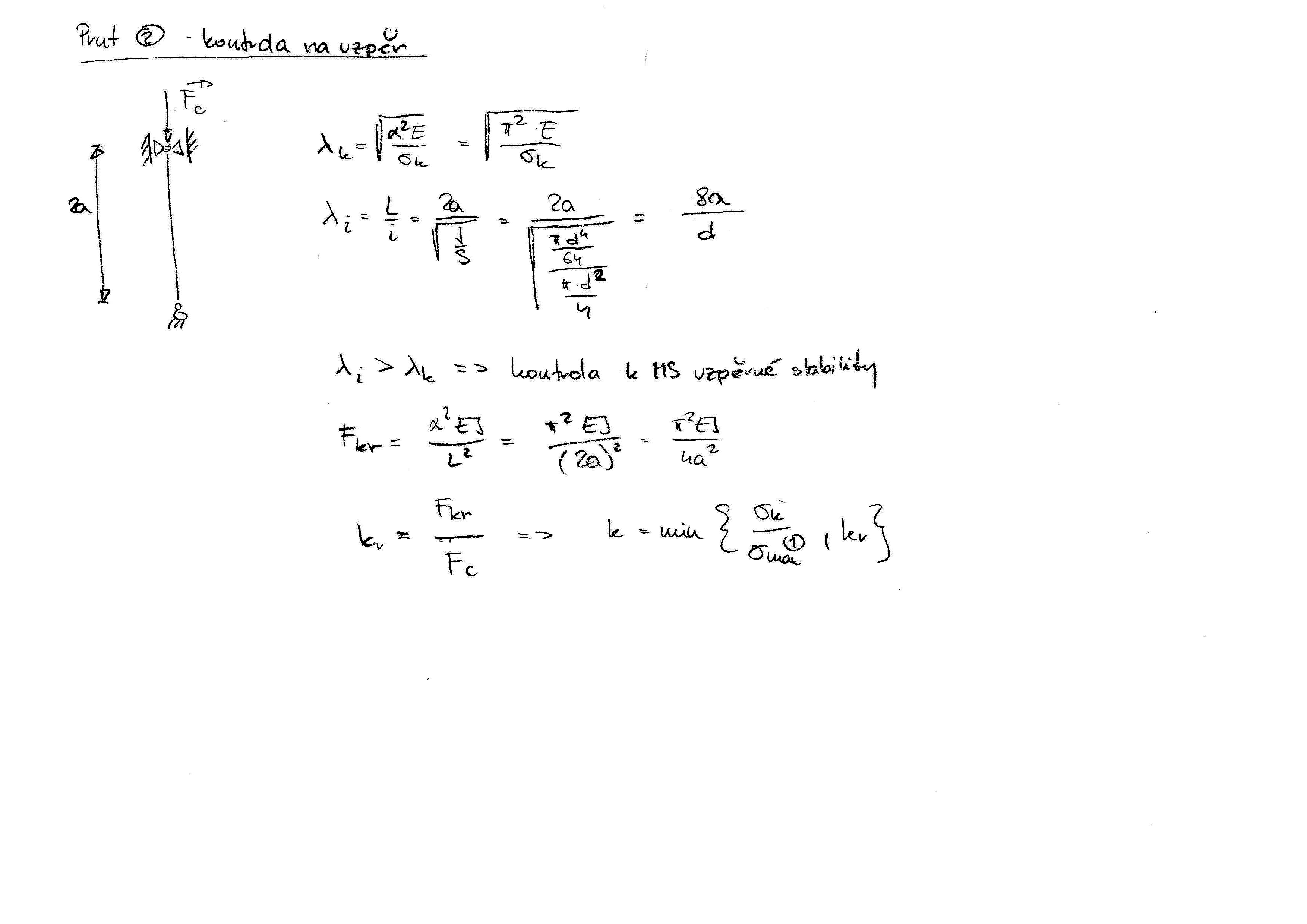
  • Mezní stav vzpěrné stability prutů (viz str. 188) - formou konkrétního příkladu, dále pak definice mezního stavu vzpěrné stability (str. 188), vztah pro kritickou sílu (vztah 9.29, str. 197), definice štíhlosti prutu (vztah 9.31, str. 198), její kritická hodnota (vztahy 9.32, 9.33, str. 199), Eulerova hyperbola (str. 198) pro tvárný/křehký materiál, doporučuji si projít demonstrační příklad na str. 201-202.

  • Napjatost v bodě tělesa (viz str. 203) - definice napjatosti (str. 203), obrázek str. 204, vztah mezi vektorem obecného napětí \(\boldsymbol{f}_\rho\) tenzorem napětí \(\boldsymbol{T}_\sigma\) a směrovými kosiny \(\boldsymbol{\alpha}\) (obecně/maticově/symbolicky, vztahy 10.6-10.8, str. 205), definice hlavní roviny (str. 207), definice invariantů a "invariantnosti" tenzoru napětí \(\boldsymbol{T}_{\sigma}\), definice oktaedrické roviny a napětí \(\tau_{o}\), rovinná napjatost (str. 218), prutová napjatost a prostý smyk (str. 222), klasifikace napjatosti (str. 223).

  • Mezní stav pružnosti (str. 226) - Trescovy podmínky plasticity (vztah 11.4, str. 227), zobrazení mezní křivky pro Tescovu podmínku plasticity v případě rovinné napjatosti (str. 228, dole), zobrazení Trescovy podmínky plasticity v Möhrově rovině (str. 229), Trescova podmínka plasticity pro případ prutové napjatosti (vztah 11.7, str. 229), Trescova podmínka plasticity pro případ smykové napjatosti (vztah 11.9, str. 229), definice podmínky plasticity HMH (vztah 11.13, str. 230), zobrazení mezní křivky pro HMH podmínku plasticity v případě rovinné napjatosti (str. 231, dole), zobrazení HMH podmínky plasticity v Möhrově rovině a definice Lodeho parametru \(\mu_\sigma\) (str. 232), HMH podmínka plasticity pro případ prutové napjatosti (vztah 11.17, str. 233), HMH podmínka plasticity pro případ smykové napjatosti (vztah 11.19, str. 233).

  • Mezní stav křehké pružnosti (nebude vyžadován u testu - přesto doporučuji k nastudování, od str. 237) - podmínka mezního stavu křehké pevnosti MOS (vztah 11.31, str. 237), grafické znázornění podmínky křehké pevnosti MOS v Möhrově rovině (str. 239).

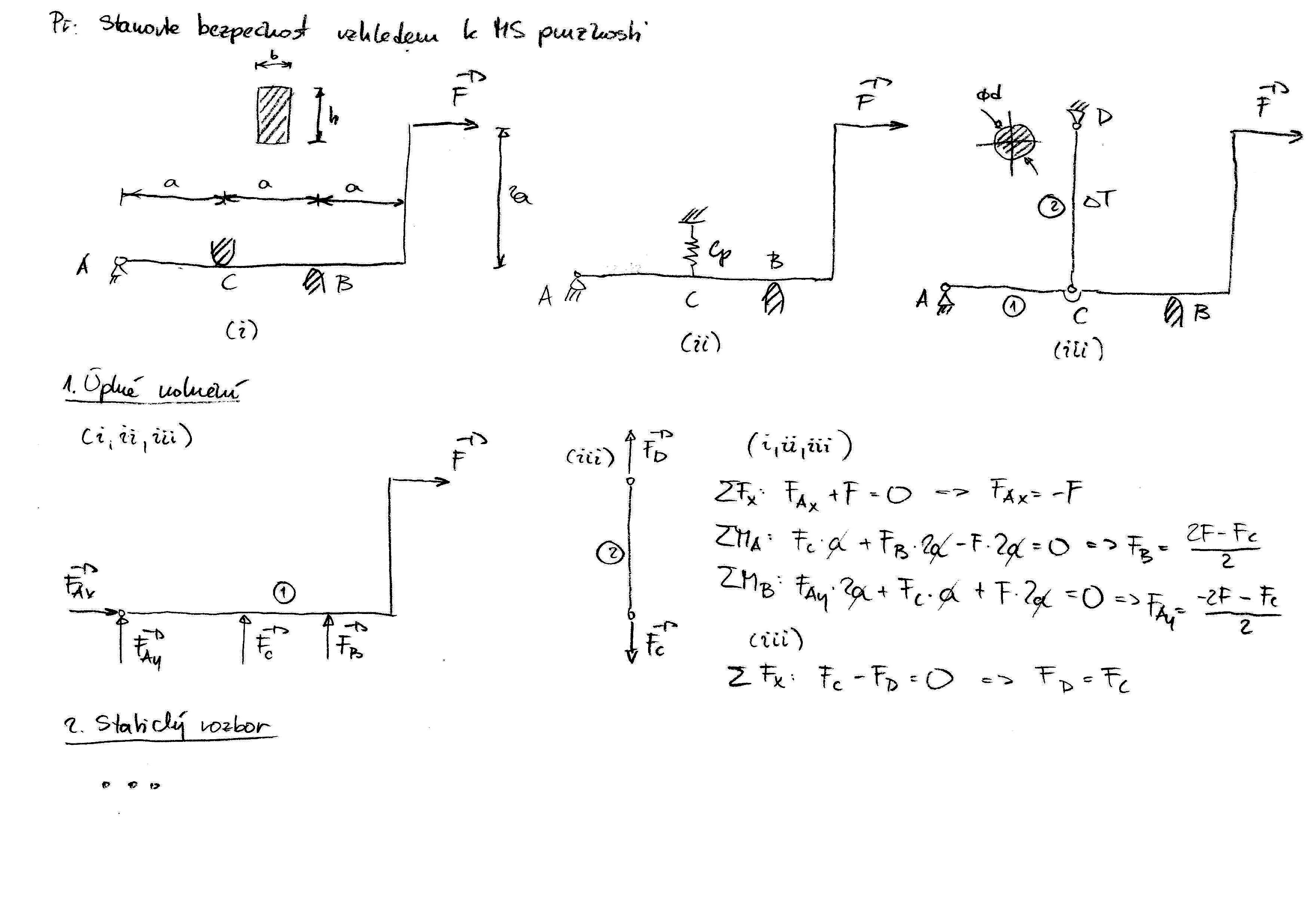
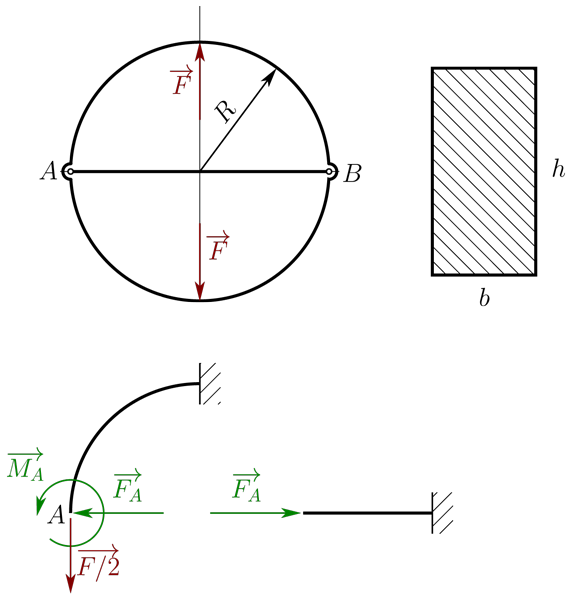
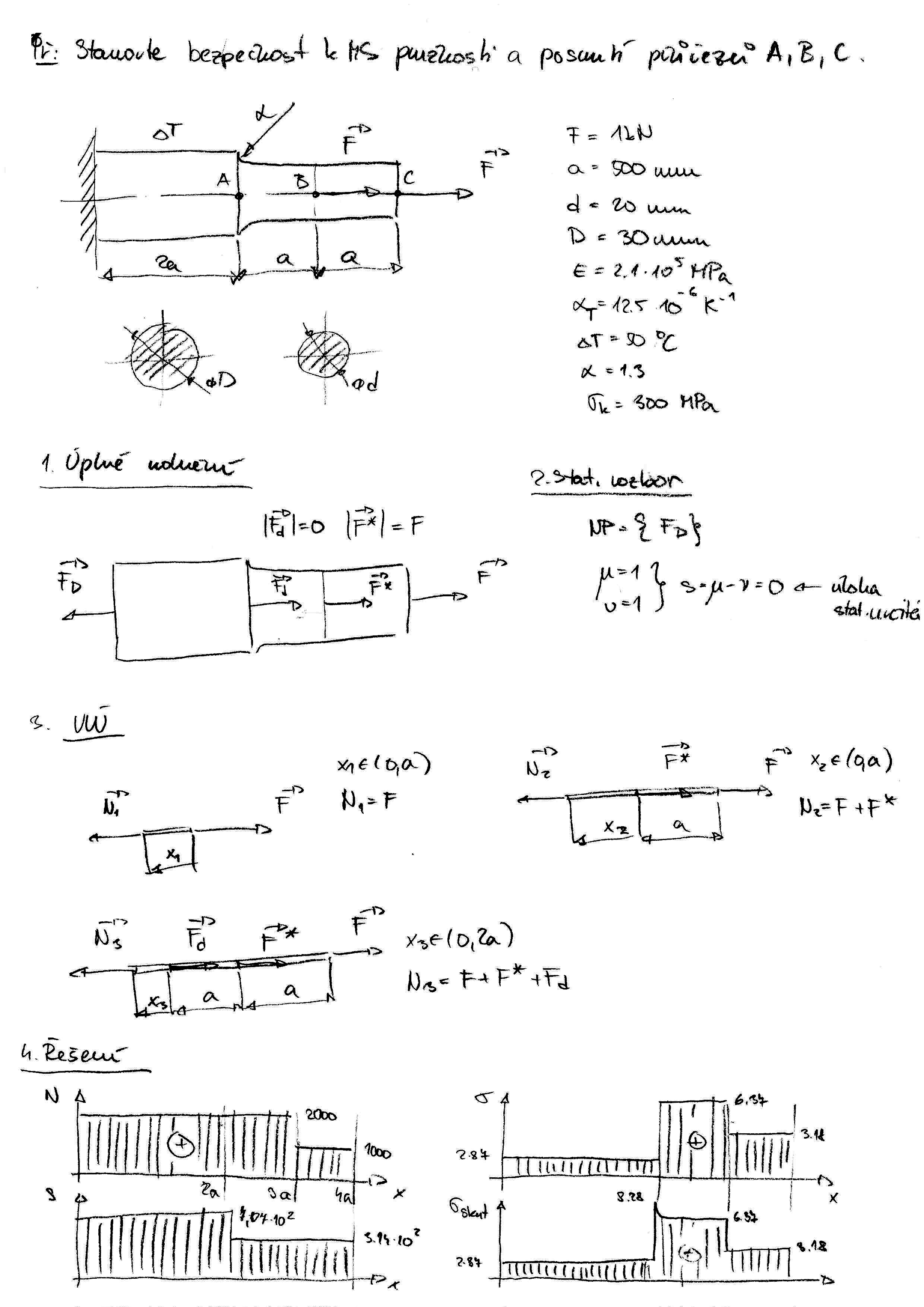
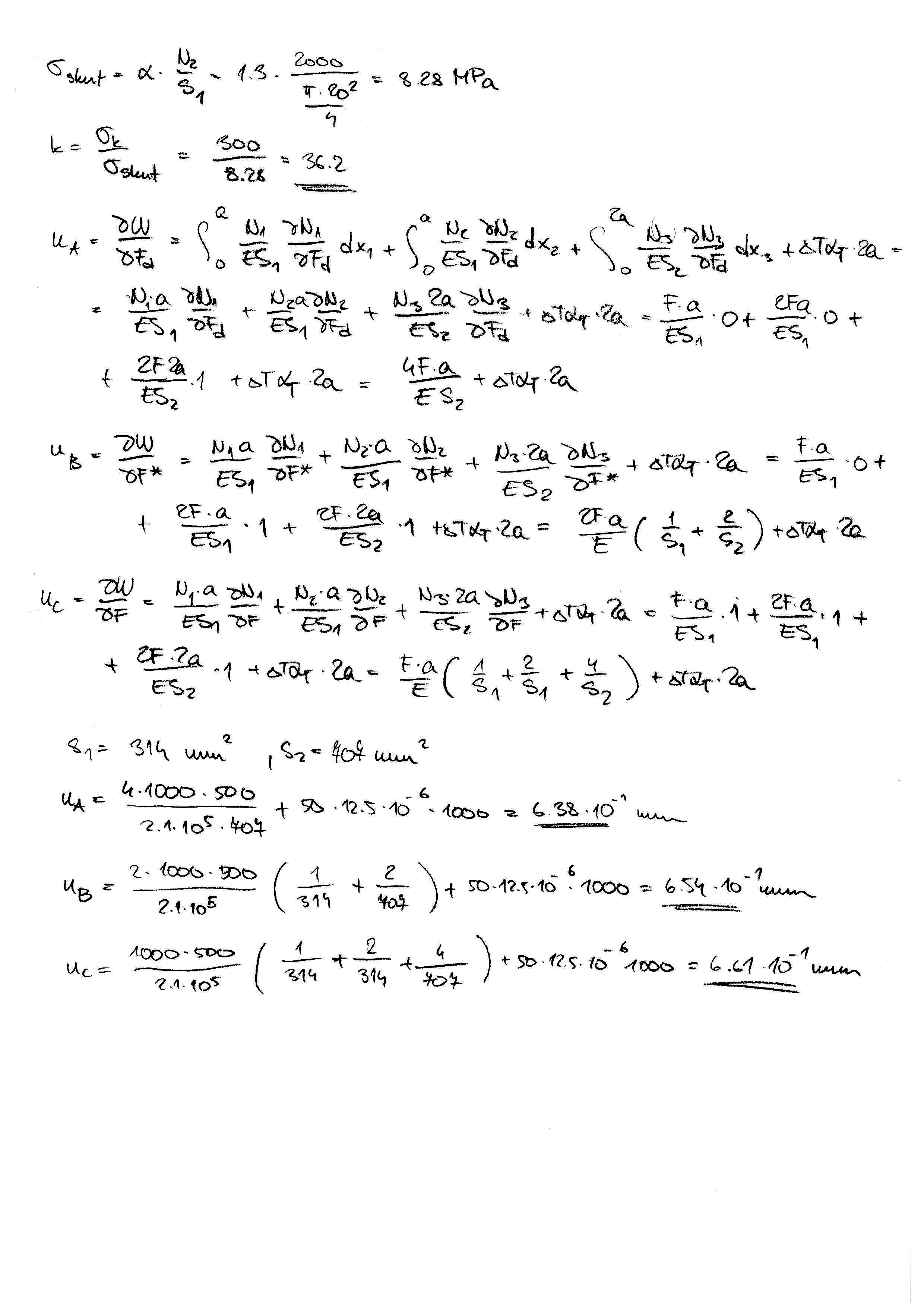
  • Součástí testu může být jednoduchý příklad staticky určitě uloženého prutu s úkolem určení extrémních hodnot napětí, příp. hodnot posuvů nebo natočení v daném bodě střednice nebo styčníku.

Příklady (\(\boldsymbol{2\times30}\) bodů) - dva příklady \(1\times\) staticky neurčitě uložených prutů nebo soustavy prutů zatížených prostým tahem/tlakem, ohybem nebo krutem.

Podklady ke stažení

Pružnost a pevnost II

Podobně jako v případě příkladů z Pružnosti a pevnosti I jsou ukázkové příklady z Pružnosti a pevnosti II ve formátu *.ipynb. Jde o soubory použitelné v systému Jupyter, který si můžete stáhnout na stránkách jupyter.org. Některé vztahy pro rotačně symetrická tělesa lze nalézt zde.

  • Cvičení 1: Kombinované namáhání.

    • Příklad v jazyce Python - Př.1. Odpovídající soubor v Jupyteru lze stáhnout zde. Obrázek lze stáhnout zde.

    • Příklad v jazyce Python - Př.2. Odpovídající soubor v Jupyteru lze stáhnout zde. Obrázek lze stáhnout zde

    • Příklad v jazyce Python - Př.3. Odpovídající soubor v Jupyteru lze stáhnout a zde. Obrázek lze stáhnout zde.

    • Ručně řešený příklad Př.4 lze stáhnout zde.

    • Ručně řešený příklad Př.5 lze stáhnout zde.

    • Ručně řešený příklad Př.6 lze stáhnout zde.

    • Ručně řešený příklad Př.7 lze stáhnout zde.

  • Cvičení 2: Napětí v bodě.

    • Příklad v jazyce Python - Př.1. Odpovídající soubor v Jupyteru lze stáhnout zde.

    • Příklad v jazyce Python - Př.2. Odpovídající soubor v Jupyteru lze stáhnout zde.

    • Ručně řešený příklad Př.3 lze stáhnout zde.

    • Ručně řešený příklad Př.4 lze stáhnout zde.

    • Ručně řešený příklad Př.5 lze stáhnout zde.

    • Ručně řešený příklad Př.6 lze stáhnout zde.

    • Ručně řešený příklad Př.7 lze stáhnout zde.

    • Ručně řešený příklad Př.8 lze stáhnout zde.

    • Ručně řešený příklad Př.9 lze stáhnout zde.

    • Ručně řešený příklad Př.10 lze stáhnout zde.

    • Ručně řešený příklad Př.11 lze stáhnout zde.

    • Ručně řešený příklad Př.12 lze stáhnout zde.

  • Cvičení 3: Trhlina v prutu.

    • Příklad v jazyce Python - Př.1. Odpovídající soubor v Jupyteru lze stáhnout zde. Obrázek lze stáhnout zde.

    • Ručně řešený příklad Př.2 lze stáhnout zde.

    • Ručně řešený příklad Př.3 lze stáhnout zde.

    • Ručně řešený příklad Př.4 lze stáhnout zde.

    • Ručně řešený příklad Př.5 lze stáhnout zde.

  • Cvičení 4: Cyklické zatěžování prutu.

    • Kratičký úvod lze stáhnout zde.

    • Ručně řešený příklad Př.1 lze stáhnout zde.

    • Ručně řešený příklad Př.2 lze stáhnout zde.

    • Ručně řešený příklad Př.3 lze stáhnout zde.

    • Ručně řešený příklad Př.4 lze stáhnout zde.

    • Ručně řešený příklad Př.5 lze stáhnout zde.

    • Ručně řešený příklad Př.6 lze stáhnout zde.

    • Ručně řešený příklad Př.7 lze stáhnout zde.

    • Ručně řešený příklad Př.8 lze stáhnout zde.

    • Ručně řešený příklad Př.9 lze stáhnout zde.

    • Ručně řešený příklad Př.10 lze stáhnout zde.

    • Ručně řešený příklad Př.11 lze stáhnout zde.

    • Ručně řešený příklad Př.12 lze stáhnout zde.

  • Cvičení 5: Válcové těleso.

    • Ručně řešený příklad Př.1 lze stáhnout zde.

    • Ručně řešený příklad Př.2 lze stáhnout zde.

    • Ručně řešený příklad Př.3 lze stáhnout zde.

    • Ručně řešený příklad Př.4 lze stáhnout zde.

    • Ručně řešený příklad Př.5 lze stáhnout zde.

    • Ručně řešený příklad Př.6 lze stáhnout zde.

    • Ručně řešený příklad Př.7 lze stáhnout zde.

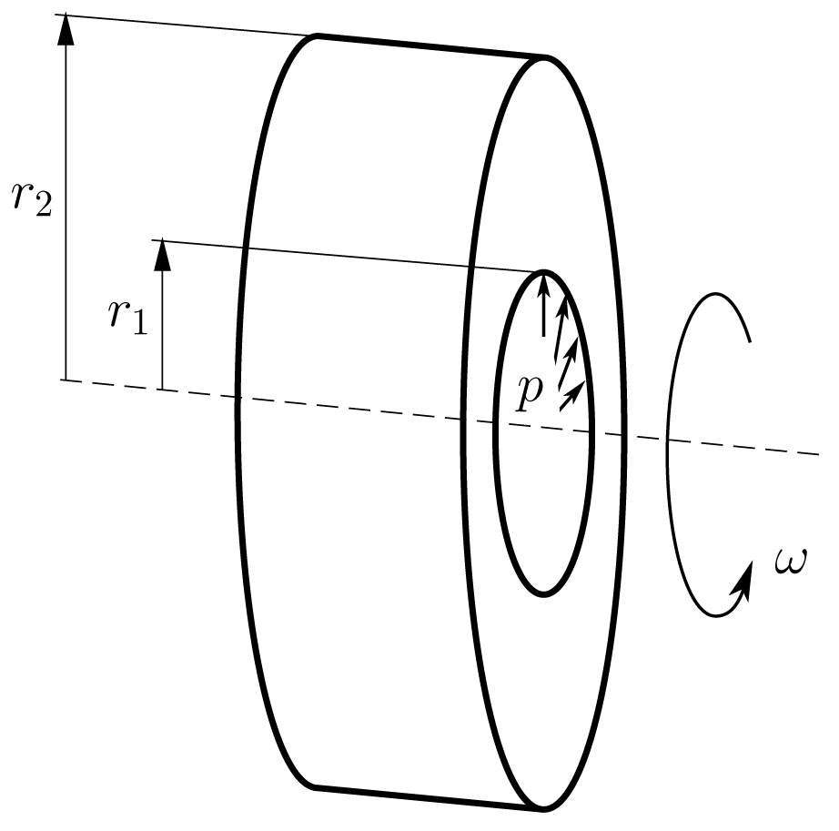
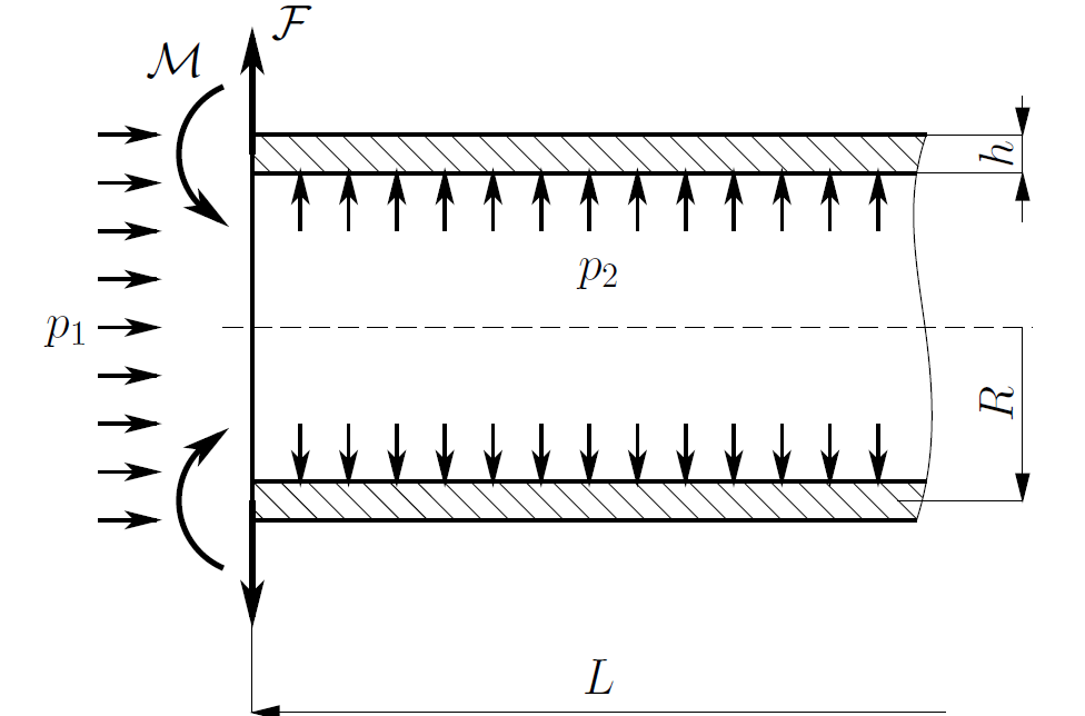
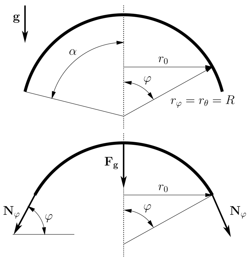
  • Cvičení 6: Rotující stěna.

    • Příklad v jazyce Python - Př.1. Odpovídající soubor v Jupyteru lze stáhnout zde. Obrázek lze stáhnout zde.

    • Příklad v jazyce Python - Př.2. Odpovídající soubor v Jupyteru lze stáhnout zde. Obrázek lze stáhnout zde.

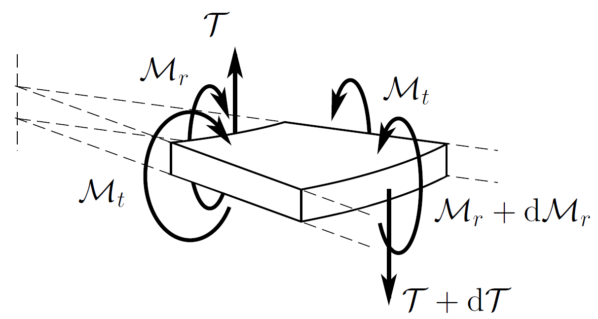
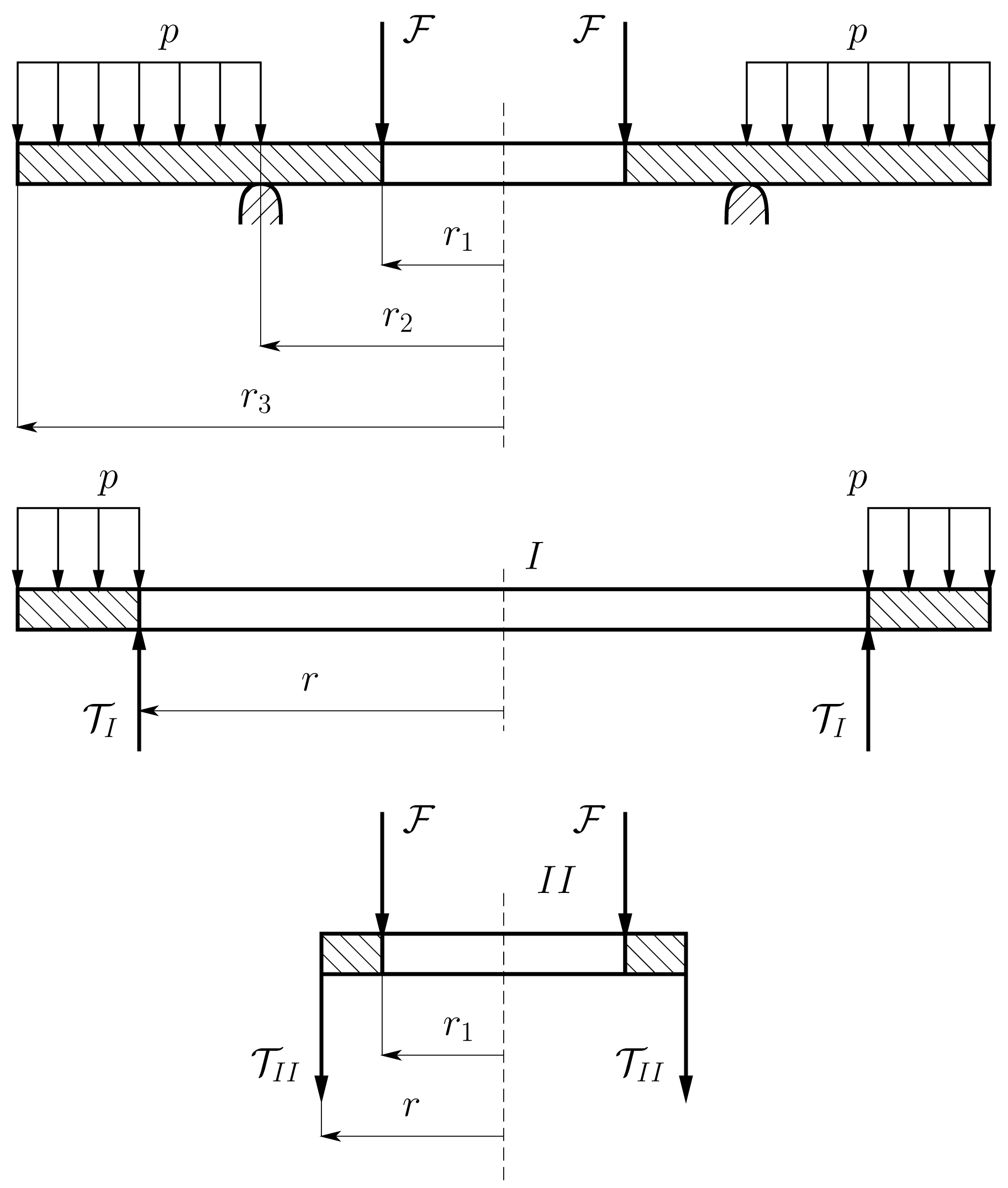
  • Cvičení 7: Průhyb rotačně symetrické desky.

    • Příklad v jazyce Python - Př.1. Odpovídající soubor v Jupyteru lze stáhnout zde. Obrázky lze stáhnout zde a zde.

    • Ručně řešený příklad Př.2 lze stáhnout zde.

    • Ručně řešený příklad Př.3 lze stáhnout zde.

    • Ručně řešený příklad Př.4 lze stáhnout zde.

    • Ručně řešený příklad Př.5 lze stáhnout zde.

    • Ručně řešený příklad Př.6 lze stáhnout zde.

    • Ručně řešený příklad Př.7 lze stáhnout zde.

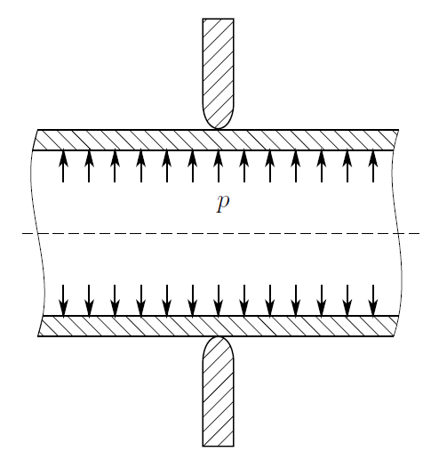
  • Cvičení 8: Dlouhá válcová skořepina.

    • Příklad v jazyce Python - Př.1. Odpovídající soubor v Jupyteru lze stáhnout zde. Obrázky lze stáhnout zde a zde.

    • Ručně řešený příklad Př.2 lze stáhnout zde.

    • Ručně řešený příklad Př.3 lze stáhnout zde.

    • Ručně řešený příklad Př.4 lze stáhnout zde.

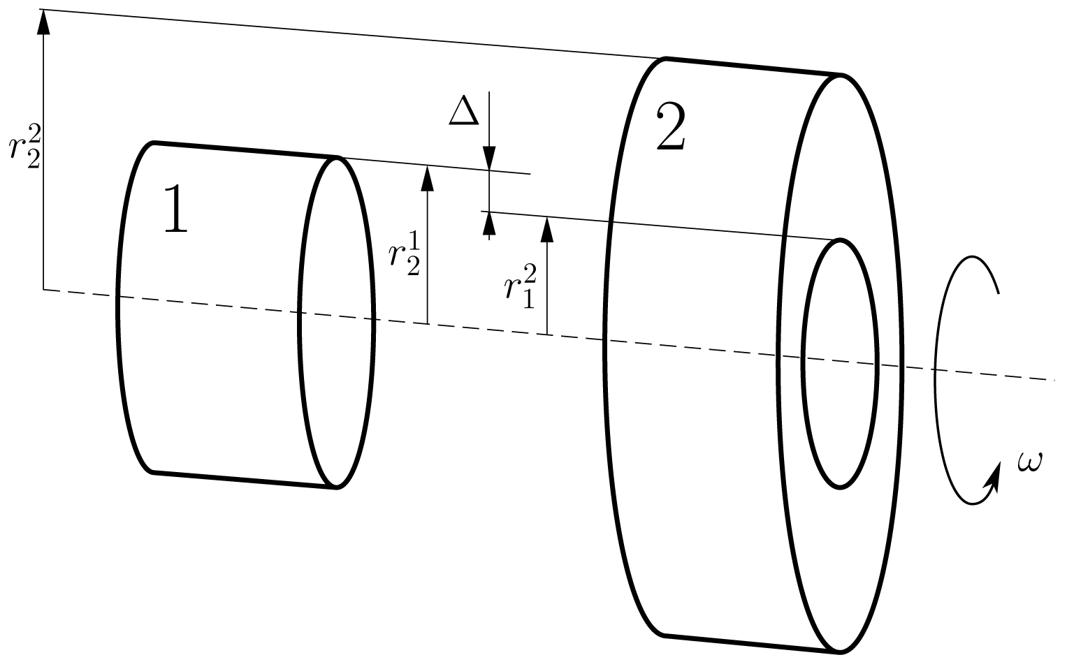
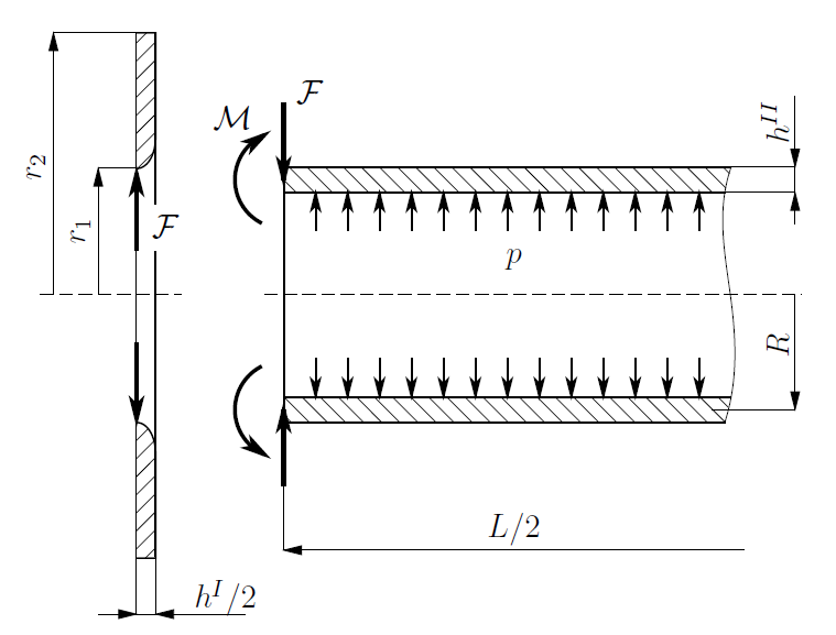
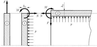
  • Cvičení 9: Složená tělesa.

    • Příklad v jazyce Python - Př.1. Odpovídající soubor v Jupyteru lze stáhnout zde. Obrázky lze stáhnout zde a zde.

    • Příklad v jazyce Python - Př.2. Odpovídající soubor v Jupyteru lze stáhnout zde. Obrázek lze stáhnout zde.

    • Ručně řešený příklad Př.3 lze stáhnout zde.

    • Ručně řešený příklad Př.4 lze stáhnout zde.

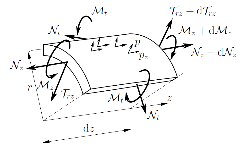
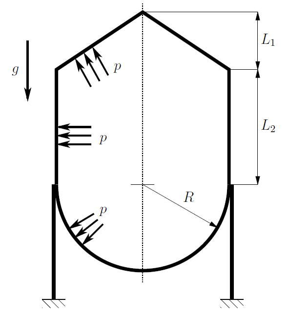
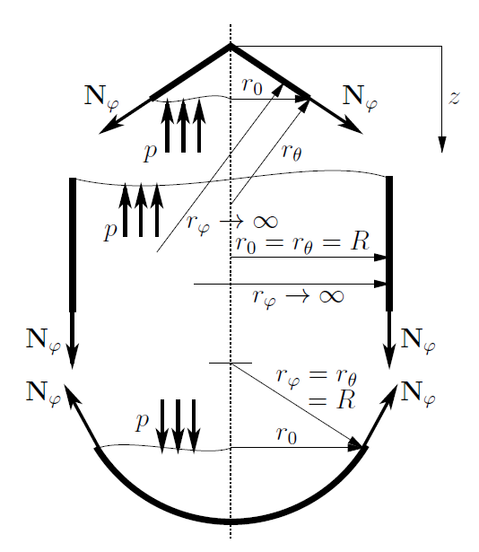
  • Cvičení 10: Bezmomentová skořepina.

    • Příklad v jazyce Python - Př.1. Odpovídající soubor v Jupyteru lze stáhnout zde. Obrázek lze stáhnout zde.

    • Příklad v jazyce Python - Př.2. Odpovídající soubor v Jupyteru lze stáhnout zde. Obrázky lze stáhnout zde a zde.

    • Ručně řešený příklad Př.3 lze stáhnout zde.

    • Ručně řešený příklad Př.4 lze stáhnout zde.

  • Cvičení 11: Metoda konečných prvků v PPI a PPII.

    • Případ krutu prizmatického prutu s nekruhovým příčným průřezem počítaný v konečnoprvkovém systému FreeFEM++ si lze prohlédnout zde.

    • Případ eliptické tenké desky (membrány) se smíšenými okrajovými podmínkami počítaný v konečnoprvkovém systému FreeFEM++ si lze prohlédnout zde.

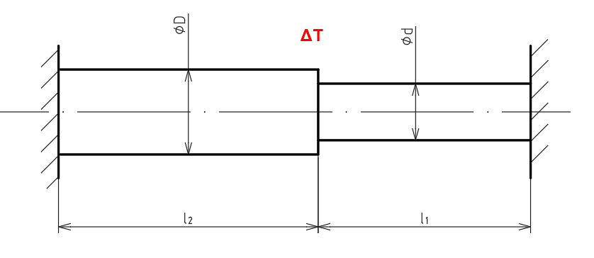
    • Případ prostého ohybu bi-materiálového prutu zatíženého změnou teploty počítaný v konečnoprvkovém systému FreeFEM++ si lze prohlédnout zde.

Continuum Mechanics

Introduction

  • Review of Equations of Mechanics: kinetics, kinematics, thermodynamic principles, constitutive equations, boundary-value problems of mechanics, equations for bar, beams, torsion and plane elasticity.

  • Bars and Beams: theory and applications.

  • Isotropic Plane Elasticity: Muskhelishvili's complex potentials, application to fracture mechanics.

  • Anisotropic Plane Elasticity: LES formalism, application to fracture mechanics.

  • Energy and Variational Principles: virtual work and energy principles, Hamilton's principle, energy theorems of structural mechanics, Castigliano's theorems, Betti's and Maxwell's theorems.

  • Variational Methods: Ritz's method, Galerkin's method, FEM.

References

Lecture 1

Kinetics - Stress at a Point

Forces acting on a body can be classified as internal and external. The internal forces resist the tendency of one part of the body to be separated from another part. The external bodies are those transmitted by the body. The external forces can be classified as body forces and surface forces. Body forces act on the distribution of mass inside the body. Examples of body forces are provided by the gravitational and magnetic forces. Body forces are usually measured per unit mass or unit volume of the body. Surface forces are contact forces acting on the boundary surface body. Example of surface forces are provided by applied forces on the surface of the body. Surface forces are reckoned per unit area.

Consider a body occupying the volume \(V\) and bounded by surface \(S\). The surface force per unit area acting on an elemental area \(dS\) is called the traction or stress vector acting on the element. Consider the surface force \(\boldsymbol{f}\) acting on a small portion \(\Delta S\) of the surface surface area \(S\) of the body. The stress vector at a point \(P\) on \(\Delta S\) is defined by

(1)\[\boldsymbol{t}=\lim_{\Delta S\rightarrow0}\frac{\boldsymbol{f}}{\Delta S}.\]

Since the magnitude and direction depend on the orientation of the plane that created the surface, we denote it by \(\boldsymbol{t}^{(\boldsymbol{n})}\), where \(\boldsymbol{n}\) denotes the normal to the plane. The component of \(\boldsymbol{t}\) that is in the direction of \(\boldsymbol{n}\) is called the normal stress. The component of \(\boldsymbol{t}\) that is normal to \(\boldsymbol{n}\) is called shear stress. Let \(\boldsymbol{t}^{(i)}\) denote the stress vector at point \(P\) on a plane perpendicular to \(x_{i}\)-axis, then

(2)\[\boldsymbol{t}^{(i)}=\sigma_{ij}\boldsymbol{e}_{j}\quad(i,j=1,2,3),\]

where \(\sigma_{ij}\) denotes the component of stress vector \(\boldsymbol{t}^{(i)}\) along the \(x_{j}\)-direction. The state of stress at a point is characterized, in general, by nine components of stress \(\sigma_{ij}\).

The relationship between the stress vector \(\boldsymbol{t}^{(n)}\) acting on a plane given by normal \(\boldsymbol{n}\) and the stress vectors on three planes perpendicular to the coordinate axes \(x_{j}\) is called the Cauchy stress formula

(3)\[t_{j}^{(\boldsymbol{n})}=n_{i}\sigma_{ij},\]

which can be written in matrix form as

(4)\[\begin{split}\left[\begin{array}{c} t_{1}^{(\boldsymbol{n})}\\ t_{2}^{(\boldsymbol{n})}\\ t_{3}^{(\boldsymbol{n})} \end{array}\right] =\left[\begin{array}{ccc} \sigma_{11} & \sigma_{12} & \sigma_{13}\\ \sigma_{21} & \sigma_{22} & \sigma_{23}\\ \sigma_{31} & \sigma_{32} & \sigma_{33} \end{array}\right]^{T} \left[\begin{array}{c} n_{1}\\ n_{2}\\ n_{3} \end{array}\right],\end{split}\]

where \([\cdot]^{T}\) denotes the transpose of the matrix. The normal and shearing components of the stress vector \(\boldsymbol{t}^{(\boldsymbol{n})}\) are given by

(5)\[\begin{split}t_{N}&=\boldsymbol{t}^{(\boldsymbol{n})}\cdot\boldsymbol{n}=\sigma_{ij}n_{i}n_{j}, \\ t_{S}&=\sqrt{\left|\boldsymbol{t}^{(\boldsymbol{n})}\right|^{2}-t_{N}^{2}}.\end{split}\]

When the components of stress are known in one coordinate system, it is of interest to determine the components of stress in another coordinate system. The relationship between the components of stress tensor in one coordinate system and the components in another coordinate system is known as the transormation of stress. Such transformations are useful in determining the maximum values of normal and shear stresses and the planes on which they act. Consider two sets of orthogonal coordinate systems \((x_1,x_2,x_3)\) and \((x_1^\prime,x_2^\prime,x_3^\prime)\). Let \((\boldsymbol{e}_1,\boldsymbol{e}_2,\boldsymbol{e}_3)\) and \((\boldsymbol{e}_1^\prime,\boldsymbol{e}_2^\prime,\boldsymbol{e}_3^\prime)\) denote the sets of basis vectors in the two coordinate systems. Suppose that the two coordinate systems are related by the transformation equation

(6)\[\boldsymbol{e}_i^\prime=a_{ij}\boldsymbol{e}_j,\]

where \(a_{ij}\) denote the directions cosines

(7)\[a_{ij}=\boldsymbol{e}_i^\prime\cdot\boldsymbol{e}_j.\]

We note that the stress dyadic

(8)\[\boldsymbol{\sigma}=\boldsymbol{e}_i\sigma_{ij}\boldsymbol{e}_j\]

at a point is invariant, that is does not depend on the coordinate system. However, the components do depend on the coordinate system. We have

(9)\[\begin{split}\boldsymbol{\sigma}&=\sigma_{ij}\boldsymbol{e}_i\boldsymbol{e}_j \\ &=\sigma_{ij}^\prime\boldsymbol{e}_i^\prime\boldsymbol{e}_j^\prime\end{split}\]

and

(10)\[(\sigma_{ij}-\sigma_{kl}^\prime a_{ki}a_{lj})\boldsymbol{e}_i\boldsymbol{e}_j=0.\]

From which follows

(11)\[\sigma_{ij}=\sigma_{kl}^\prime a_{ki}a_{lj}.\]

The question of finding the maximum and minimum normal stresses, called principal stresses, at a point is the considerable interest. The maximum normal stress at a point acts in a plane on which the shear stress is zero and consequently

(12)\[\boldsymbol{t}^{(\boldsymbol{n})}=\lambda\boldsymbol{n},\]

where \(\lambda\) denotes the magnitude of the normal stress and \(\boldsymbol{n}\) denotes the unit normal to the plane on which the maximum stress is acting. This formula can also be written as

(13)\[\boldsymbol{t}^{(\boldsymbol{n})}=\boldsymbol{\sigma}\cdot\boldsymbol{n}.\]

Equating these two equations, we obtain

(14)\[\boldsymbol{\sigma}\cdot\boldsymbol{n}-\lambda\boldsymbol{n}=0\]

or in component form

(15)\[(\sigma_{ij}-\lambda\delta_{ij})n_j=0,\]

where \(\delta_{ij}\) is a Kronecker delta

(16)\[\begin{split}\delta_{ij}=\left\{\begin{array}{c} 0\quad\mathrm{for}\ i\neq j,\\ 1\quad\mathrm{for}\ i=j. \end{array} \right. .\end{split}\]

Equation (15) has a nontrivial solution (\(n_i\neq 0,i=1,2,3\)) only if the determinant of the coefficient matrix is zero

(17)\[\begin{split}\left|\begin{array}{ccc} \sigma_{11}-\lambda & \sigma_{12} & \sigma_{13}\\ \sigma_{21} & \sigma_{22}-\lambda & \sigma_{23}\\ \sigma_{31} & \sigma_{32} & \sigma_{33}-\lambda\\ \end{array} \right|=0.\end{split}\]

The determinant leads to the polynomial called characteristic and the three values of \(\lambda\) are called characteristic values or eigenvalues and associated (unit) normal vectors \(\boldsymbol{n}\) are called characteristic vectors or eigenvectors. The characteristic polynomial (17) is of the form

(18)\[-\lambda^3+I_1\lambda^2-I_2\lambda+I_3=0,\]

where \(I_1\), \(I_2\) and \(I_3\) are stress invariants defined as

(19)\[\begin{split}I_1 &= \sigma_{ii}=\sigma_{11}+\sigma_{22}+\sigma_{33}, \\ I_2 &= \frac{1}{2}(\sigma_{ii}\sigma_{jj}-\sigma_{ij}\sigma_{ji} \\ &= \sigma_{11}\sigma_{22}+\sigma_{22}\sigma_{33}+\sigma_{33}\sigma_{11}-(\sigma_{12}^2+\sigma_{13}^2+\sigma_{23}^2), \\ I_3 &=\det[\boldsymbol{\sigma}]=|\sigma_{ij}|.\end{split}\]

For symmetric tress dyadic \(\boldsymbol{\sigma}\), i.e. \(\sigma_{ij}=\sigma_{ji}\), the eigenvalues are real.

The equation of motion for solids can be derived from the principle of of conservation of linear momentum, which says that the time rate of change of the total momentum of a given body equals the vector sum of all the external forces acting on the body and provides the Newton's third law of action and reaction governs the internal forces. The momentum of the elemental volume \(dV\) is \((\mathrm{mass}\times\mathrm{velocity})=(\rho dV)\partial\boldsymbol{u}/\partial t\). The total momentum is given by

(20)\[\int_V \rho\frac{\partial\boldsymbol{u}}{\partial t}dV.\]

The time rate of the momentum is

(21)\[\frac{d}{dt}\int_V \rho\frac{\partial\boldsymbol{u}}{\partial t}dV= \int_V\frac{d}{dt}(\rho dV)\frac{\partial\boldsymbol{u}}{\partial t} +\int_V\rho\frac{\partial^2\boldsymbol{u}}{\partial t^2}dV,\]

where \(d/dt\) denotes the total (material) time derivative. The first integral on the right-hand side is equal to zero because of the principle of conservation of mass of a given material

(22)\[\frac{d}{dt}(\rho dV)=0.\]

The momentum principle can now be expressed as

(23)\[\int_V\rho\frac{\partial^2\boldsymbol{u}}{\partial t^2}dV=\int_V\boldsymbol{f}dV -\int_S\boldsymbol{t}dS.\]

Using equation (13), the stress vector \(\boldsymbol{t}\) can be expressed in terms of the stress tensor (dyadic) \(\boldsymbol{\sigma}\) and unit normal \(\boldsymbol{n}\). We obtain

(24)\[\int_V\rho\frac{\partial^2\boldsymbol{u}}{\partial t^2}dV -\int_V\boldsymbol{f}dV -\int_S\boldsymbol{\sigma}\cdot\boldsymbol{n}dS=0\]

Using the divergence theorem, the surface integral can be converted to a volume integral

(25)\[-\int_V\left(\Delta\cdot\boldsymbol{\sigma}+\boldsymbol{f} -\frac{\partial^2\boldsymbol{u}}{\partial t^2}dV\right)dV=0.\]

The equation should hold for arbitrary region \(V\). This implies that the integrand of the left-hand side of (25) should be identically equal to zero. This gives the vector from of the equation of motion

(26)\[\Delta\cdot\boldsymbol{\sigma}+\boldsymbol{f} =\frac{\partial^2\boldsymbol{u}}{\partial t^2}.\]

In a rectangular cartesian coordinate system, this equation takes the form

(27)\[\frac{\partial\sigma_{ij}}{\partial x_j}+f_i=\rho\frac{\partial^2u_i}{\partial t^2}.\]

The equation of equilibrium are obtained by setting the right-hand side of (26) equal to zero

(28)\[\Delta\cdot\boldsymbol{\sigma}+\boldsymbol{f}=\boldsymbol{0}.\]

When a body is not subjected to distributed couples (i.e., volume-dependent couples are not present), one can establish the symmetry of the stress tensor using the Newton's second law for moments or using the principle of moment of momentum. Both methods give the result

(29)\[\epsilon_{ijk}\sigma_{ij}=0\quad\mathrm{for}\ k=1,2,3,\]

where \(\epsilon_{ijk}\) is the permutation symbol

(30)\[\begin{split}\epsilon_{ijk}=\left\{\begin{array}{cl} 1 & \mathrm{if}\ ijk\ \mathrm{are}\ \mathrm{in}\ \mathrm{cyclic}\ \mathrm{order}\\ & \mathrm{and}\ \mathrm{are}\ \mathrm{no}\ \mathrm{repeated}\ (i\neq j\neq k), \\ -1 & \mathrm{if}\ ijk\ \mathrm{are}\ \mathrm{not}\ \mathrm{in}\ \mathrm{cyclic}\ \mathrm{order}\\ & \mathrm{and}\ \mathrm{are}\ \mathrm{no}\ \mathrm{repeated}\ (i\neq j\neq k), \\ 0 & \mathrm{if}\ \mathrm{any}\ \mathrm{of}\ ijk\ \mathrm{are}\ \mathrm{repeated}. \end{array}\right.\end{split}\]

Or rewritten to the components

(31)\[\begin{split}\begin{array}{ll} k=1: & \sigma_{23}-\sigma_{32}=0 \\ k=2: & \sigma_{31}-\sigma_{13}=0 \\ k=3: & \sigma_{12}-\sigma_{21}=0. \end{array}\end{split}\]

Thus, there are only six stress components that are independent. Because (26) contains three equations relating six stress components, the equations of equilibrium are not sufficient for the determination of the stress components. Additional equations are required, the strain-displacement equations and constitutive equations.

  • Examples 1:

    • Example 1.1 to download here and here.

    • Example 1.2 to download here.

    • Example 1.3 to download here and here.

Lecture 2

Kinematics - Strain at a Point

To describe the motion of a deformable body, we establish a fixed reference frame in three dimensional space and denote the Cartesian coordinates of a point be \(\boldsymbol{x}=(x_1,x_2,x_3)\). A measure of the deformation in a body is provided by the change in the distance between points in the body. Consider two neighboring points \(P=(x_1,x_2,x_3)\) and \(Q=(x1+dx_1,x_2+dx_2,x_3+dx_3)\) in the reference configuration. Under the action of externally applied forces, the body deforms and the points \(P\) and \(Q\) move to new places \(\overline{P}=(\xi_1,\xi_2,\xi_3)\) and \(\overline{Q}=(\xi_1+d\xi_1,\xi_2+d\xi_2,\xi_3+d\xi_3)\), respectively. Since points \(P\) and \(Q\) are arbitrary, the discussion applies to any point in the body. The motion of a particle occupying position \(\boldsymbol{x}\) in the undeformed body to point \(\boldsymbol{\xi}\) in the deformed body can be expressed by the transformation

(32)\[\xi_i=\xi_i(x_1,x_2,x_3,t),\]

where \(t\) denotes time. By assumption a continuous medium cannot have gaps or overlaps. Therefore, a one-to-one correspondence exists between points in the undeformed body and points in the deformed body. Consequently, a unique inverse to (32) holds

(33)\[x_i=x_i(\xi_1,\xi_2,\xi_3,t).\]

IF the distances between points \(P\) and \(Q\) is \(dS\) and the distance between points \(\overline{P}\) and \(\overline{Q}\) is \(d\overline{S}\), then the measure of deformation of the body is

(34)\[\begin{split}(d\overline{S})^2-(dS)^2 &= d\xi_id\xi_i-dx_idx_i \\ &= 2\varepsilon_{ij}dx_idx_j,\end{split}\]

where \(\varepsilon_{ij}\) are the components of the Green strain tensor at point \(P\)

(35)\[\varepsilon_{ij}=\left(\frac{\partial\xi_m}{\partial x_i}\frac{\partial\xi_m}{\partial x_j}-\delta_{ij}\right)dx_idx_j.\]

The symbol \(\delta_{ij}\) is a Kronecker delta (16). The displacements can be written as

(36)\[u_m=\xi_m-x_m\Rightarrow\frac{\partial\xi_m}{\partial x_i}=\frac{\partial u_m}{\partial x_i}+\delta_{mi}.\]

The substitution of the last expression to (35) gives the expression of strains in terms of the displacements at point \(P\)

(37)\[\varepsilon_{ij}=\frac{1}{2}\left(\frac{\partial u_i}{\partial x_j}+\frac{\partial u_j}{\partial x_i} +\frac{\partial u_m}{\partial x_j}\frac{\partial u_m}{\partial x_j}\right).\]

We will assume in the following that the displacement components are small compared to unity, i.e.

(38)\[\frac{\partial u_i}{\partial x_j}\ll 1,\quad\left(\frac{\partial u_i}{\partial x_j}\right)^2\approx 0,\]

then then strain components \(\varepsilon_{ij}\) become the infinitesimal strain componets

(39)\[e_{ij}=\frac{1}{2}\left(\frac{\partial u_i}{\partial x_j}+\frac{\partial u_j}{\partial x_i}\right).\]

Similarly to the stresses at a point, it is a matter of interest to know the components of strain at a point in one coordinate system, e.g. \((x_1^\prime,x_2^\prime,x_3^\prime)\), if they are known in the another coordinate system \((x_1,x_2,x_3)\) at the same point. It not difficult to proof, that the tensor character of strain is associated with the transformation relation

(40)\[\varepsilon_{ij}^\prime=a_{im}a_{jn}\varepsilon_{mn},\]

where

(41)\[a_{ij}=\boldsymbol{e}_i^\prime\cdot\boldsymbol{e}_j.\]

When the strain components are given, the determination of the displacements is not always possible, because there are six strain components related to three displacement components. Stated in other words, there are six differential equations involving three unknowns. Thus, the six equations should be compatible with each other in the sense that any three equations should give the same displacement field. Assuming the infinitesimal strain components, the only way, how to connect six partial differential equation (39) and eliminate the components of displacements appearing in them, is to derive them two times. Then it can be observed

(42)\[e_{ij,kl}+e_{kl,ij}=e_{lj,ki}+e_{ki,lj}.\]

Equation (42) forms the necessary and sufficient conditions for the existence of a single-valued displacement field (when the strains are given). It is 81 equations, but only six of them are non trivial and different and linearly independent from each other

(43)\[\begin{split}\frac{\partial^2e_{11}}{\partial x_2^2}+\frac{\partial^2e_{22}}{\partial x_1^2} &= 2\frac{\partial^2e_{12}}{\partial x_1\partial x_2}, \\ \frac{\partial^2e_{22}}{\partial x_3^2}+\frac{\partial^2e_{33}}{\partial x_2^2} &= 2\frac{\partial^2e_{23}}{\partial x_2\partial x_3} ,\\ \frac{\partial^2e_{11}}{\partial x_3^2}+\frac{\partial^2e_{33}}{\partial x_1^2} &= 2\frac{\partial^2e_{13}}{\partial x_1\partial x_3},\end{split}\]
(44)\[\begin{split}\frac{\partial}{\partial x_1}\left(-\frac{\partial e_{23}}{\partial x_1} +\frac{\partial e_{13}}{\partial x_2} +\frac{\partial e_{12}}{\partial x_3}\right) & = \frac{\partial^2e_{11}}{\partial x_2\partial x_3}, \\ \frac{\partial}{\partial x_2}\left(-\frac{\partial e_{13}}{\partial x_2} +\frac{\partial e_{12}}{\partial x_3} +\frac{\partial e_{23}}{\partial x_1}\right) & = \frac{\partial^2e_{22}}{\partial x_1\partial x_3}, \\ \frac{\partial}{\partial x_3}\left(-\frac{\partial e_{12}}{\partial x_3} +\frac{\partial e_{23}}{\partial x_1} +\frac{\partial e_{13}}{\partial x_2}\right) & = \frac{\partial^2e_{33}}{\partial x_1\partial x_2}.\end{split}\]
  • Examples 2:

Lecture 3

First Law of Thermodynamics

The first law of thermodynamics is commonly known as the principle of balance of energy and it can be regarded as a statement of the interconvertibility of heat and work. The law does not place any restriction on the direction of the process. The first law of thermodynamics states that the time-rate of change of the total energy (i.e. sum of the kinetic energy and the internal energy) is equal to the sum of the rate of work done by the external forces and the change of heat content per unit time

(45)\[\frac{d}{dt}(K+U)=W+H,\]

where \(K\) denotes the kinetic energy, \(U\) is the internal energy, \(W\) is the power input and \(H\) is the heat input to the system. The kinetic energy of the system is given by

(46)\[K=\int_V \rho\frac{\partial\boldsymbol{u}}{\partial t}\cdot\frac{\partial\boldsymbol{u}}{\partial t}dV.\]

If \(\hat{U}_0\) is the energy per unit mass (or specific internal energy), the total internal energy of the system is given by

(47)\[U=\int_V\rho \hat{U}_0dV.\]

The kinetic energy \(K\) of a system is the energy associated with the macroscopically observable velocity of the continuum. The kinetic energy associated with the microscopic motions of molecules of the continuum is a part of the internal energy. The elastic strain energy and other forms of energy are also parts of internal energy.

The power input in the nonpolar case, consists of the rate at which the external surface tractions \(\boldsymbol{t}\) per unit area and body \(\boldsymbol{f}\) per unit volume are doing work on the mass system instantaneously occupying the volume \(V\) bounded by \(S\)

(48)\[\begin{split}W &= \int_S\boldsymbol{t}\cdot\frac{\partial\boldsymbol{u}}{\partial t}dS +\int_V\boldsymbol{f}\cdot\frac{\partial\boldsymbol{u}}{\partial t}dV \\ &= \int_S(\boldsymbol{n}\cdot\boldsymbol{\sigma}\cdot\frac{\partial\boldsymbol{u}}{\partial t}dS +\int_V\boldsymbol{f}\cdot\frac{\partial\boldsymbol{u}}{\partial t}dV \\ &= \int_V\left[\nabla\cdot\left(\boldsymbol{\sigma}\cdot\frac{\partial\boldsymbol{u}}{\partial t}\right) +\boldsymbol{f}\cdot\frac{\partial\boldsymbol{u}}{\partial t}\right]dV \\ &= \int_V\left[(\nabla\cdot\boldsymbol{\sigma}+\boldsymbol{f})\cdot\frac{\partial\boldsymbol{u}}{\partial t} +\boldsymbol{\sigma}:\nabla\frac{\partial\boldsymbol{u}}{\partial t}\right]dV,\end{split}\]

where \(:\) denotes the double-dot product of tensors. The expression (48) can be rewritten to the form

(49)\[W=\frac{d}{dt}\int_V\frac{\rho}{2}\frac{\partial u_i}{\partial t}\frac{\partial u_i}{\partial t}dV +\int_V\sigma_{ij}\dot{e}_{ij}dV.\]

The rate of heat input consists of conduction through the surface \(S\) and internal heat generation in the body

(50)\[H=-\int_S\boldsymbol{q}\cdot\boldsymbol{n}dS+\int_V\rho QdV,\]

where \(\boldsymbol{q}\) is the heat flux vector normal to the surface and \(Q\) is the internal heat source per mass. Substituting (46), (47), (49) and (50) into (45), we obtain

(51)\[\frac{d}{dt}\int_V\rho \hat{U}_0dV=\int_V\sigma_{ij}\dot{e}_{ij}dV-\int_S q_in_idS+\int_V\rho QdV,\]

or

(52)\[\int_V\left(\rho\frac{\partial \hat{U}_0}{\partial t}-\sigma_{ij}\dot{e}_{ij} +\frac{\partial q_i}{\partial x_i}-\rho Q\right)dV=0\]

for arbitrary volume \(V\). Thus the conservation of energy implied by the first law of thermodynamics is given

(53)\[\rho\frac{\partial \hat{U}_0}{\partial t}=\sigma_{ij}\dot{e}_{ij}+\rho Q-\frac{\partial q_i}{\partial x_i}.\]

Second Law of Thermodynamics

From our experience we know, that mechanical energy that is converted into heat cannot be converted back into mechanical energy. Although the first law of thermodynamics does not restrict the reversal process, namely the conversion of heat to internal energy and internal energy to motion, such a reversal cannot occur because the frictional dissipation is an irreversible process. In addition to the first, the second law adopts these features. The second law of thermodynamics for a reversible process states, that there exits a function \(\eta=\eta(e_{ij},T)\) called the specific entropy, such that

(54)\[d\eta=\left[-\frac{1}{\rho}\nabla\cdot\left(\frac{1}{T}\boldsymbol{q}\right)+\frac{Q}{T}\right]dt\]

is a perfect differential. Equation (54) is called the entropy equation of state. Combining (53) and (54) we arrive at the equation

(55)\[\sigma_{ij}\dot{e}_{ij}+\rho T\dot{\eta}=\dot{U_0}.\]

For irreversible processes, the second law of thermodynamics states that (54) is not total differential, but

(56)\[\dot{\eta}\geq-\frac{1}{\rho}\nabla\cdot\left(\frac{1}{T}\boldsymbol{q}\right)+\frac{Q}{T},\]

which is known as the Clausius-Duhem inequality.

Lecture 4

Generalized Hook's Law

A material body is said to be ideally elastic when the body recovers (under isothermal conditions) its original form completely upon removal of the forces causing deformation and there is a one-to-one relationship between the state of stress and state of strain. The generalized Hook's law relates the nine components of stress to the nine components of strain by the linear relation

(57)\[\sigma_{ij}=c_{ijkl}e_{kl},\]

where \(e_{kl}\) are the infinitesimal strain components, \(\sigma_{ij}\) are Cauchy stress components and \(c_{ijkl}\) are the material parameters. A material is said to be homogeneous if the parameters \(c_{ijkl}\) do not vary from point to point in the body. The nine equations in (57) contain 81 parameters. However, owing to the symmetry of both \(sigma_{ij}\) and \(e_{kl}\), it follows that

(58)\[c_{ijkl}=c_{jikl},\quad c_{ijkl}=c_{ijlk}\]

and there are only 36 constants. Equation (57) can also be expressed in the matrix form

(59)\[\begin{split}\left[\begin{array}{c} \sigma_1 \\ \sigma_2 \\ \sigma_3 \\ \sigma_4 \\ \sigma_5 \\ \sigma_6 \end{array}\right] =\left[\begin{array}{cccccc} c_{11} & c_{12} & c_{13} & c_{14} & c_{15} & c_{16} \\ c_{21} & c_{22} & c_{23} & c_{24} & c_{25} & c_{26} \\ c_{31} & c_{32} & c_{33} & c_{34} & c_{35} & c_{36} \\ c_{41} & c_{42} & c_{43} & c_{44} & c_{45} & c_{46} \\ c_{51} & c_{52} & c_{53} & c_{54} & c_{55} & c_{56} \\ c_{61} & c_{62} & c_{63} & c_{64} & c_{65} & c_{66} \end{array}\right] \left[\begin{array}{c} e_1 \\ e_2 \\ e_3 \\ e_4 \\ e_5 \\ e_6 \end{array}\right]\end{split}\]

or

(60)\[\sigma_i=c_{ij}e_j,\]

where

(61)\[\begin{split}\begin{array}{ccc} \sigma_{11}=\sigma_1, & \sigma_{22}=\sigma_2, & \sigma_{33}=\sigma_3, \\ \sigma_{12}=\sigma_6, & \sigma_{13}=\sigma_5, & \sigma_{12}=\sigma_4, \end{array}\end{split}\]
(62)\[\begin{split}\begin{array}{ccc} e_{11}=e_1, & e_{22}=e_2, & e_{33}=e_3, \\ 2e_{12}=e_6, & 2e_{13}=e_5, & 2e_{12}=e_4. \end{array}\end{split}\]

Hence, the rules apply to indexes in (59) are

(63)\[\begin{split}\begin{array}{cccccc} 11\leftrightarrow 1 & 22\leftrightarrow 2 & 33\leftrightarrow 3 & 12\leftrightarrow 6 & 13\leftrightarrow 5 & 23\leftrightarrow 4 \\ 1111\leftrightarrow 11 & 1122\leftrightarrow 12 & 1133\leftrightarrow 13 & 1112\leftrightarrow 16 & 1113\leftrightarrow 15 & 1123\leftrightarrow 14 \\ \mathrm{etc.}&&&&& \end{array}\end{split}\]

Note that \(\sigma_i\) and \(e_j\) do not constitute the components of tensor. Therefore one cannot transform the components \(\sigma_i\) and \(e_i\) like vectors, but these must be rewritten to the tensor components \(\sigma_{ij}\) or \(e_{kl}\), transformed and consequently written to the vector form. The same rule is valid for matrix components \(c_{ij}\).

Strain Energy Density Function

In ideal elasticity it is assumed that all of the input work is converted into internal energy in the form of recoverable stored elastic energy. We denote the strain energy per unit volume by \(U_0=U_0(e_{ij})\). Therefore

(64)\[\frac{\partial U_0}{\partial t}=\frac{\partial U_0}{\partial e_{ij}}\frac{\partial e_{ij}}{\partial t}.\]

The specific internal energy \(\hat{U}_0\) is related to the strain energy density \(U_0\) by relation

(65)\[U_0=\rho\hat{U}_0.\]

Substituting (64) into the energy equation (53) and putting \(Q=q_i=0\) for isothermal case, we get

(66)\[\frac{\partial U_0}{\partial e_{ij}}\dot{e}_{ij}=\sigma_{ij}\dot{e}_{ij}\]

from which follows

(67)\[\sigma_{ij}=\frac{\partial U_0}{\partial e_{ij}}.\]

When temperature effects are involved, the strain energy density is a function of strains and temperature \(U_0=U_0(e_{ij},T)\) and it must be introduced the free-energy function \(\Psi(e_{ij},T)\) combining the strain energy density and entropy

(68)\[\rho\Psi=U_0(e_{ij},T)-\rho T\eta(e_{ij},T).\]

Since \(\Psi\) is a function of the strains and temperature, we have

(69)\[\dot{U}_0=\rho\frac{\partial\Psi}{\partial e_{ij}}\dot{e}_{ij} +\left(\rho\frac{\partial\Psi}{\partial T}+\rho\eta\right)\dot{T} +\rho T\dot{\eta}.\]

Substituting (55) into (69) yields

(70)\[0=\left(\rho\frac{\partial\Psi}{\partial e_{ij}}-\sigma_{ij}\right)\dot{e}_{ij} +\rho\left(\frac{\partial\Psi}{\partial T}+\eta\right)\dot{T}.\]

Since \(\dot{e}_{ij}\) and \(\dot{T}\) are independent of each other, it follows that

(71)\[\sigma_{ij}=\rho\frac{\partial\Psi}{\partial e_{ij}},\quad\eta=-\frac{\partial\Psi}{\partial T}.\]

If the deformation process is isothermal and reversible, we have

(72)\[\Psi=\Psi(e_{ij})\]

and hence \(\eta=0\) and from (67) and (71) we get

(73)\[\rho d\Psi=dU_0=\sigma_{ij}de_{ij}.\]

This equation can be used to reduce the number of independent elastic constants to 21. The substitution of the generalized Hook's law (57) into the first relation of (71) gives

(74)\[\rho\frac{\partial\Psi}{\partial e_{ij}}=c_{ijkl}e_{kl}.\]

The partial differentiation of (74) with respect to \(e_{kl}\) gives

(75)\[\rho\frac{\partial}{\partial e_{kl}}\left(\frac{\partial\Psi}{\partial e_{ij}}\right)=c_{ijkl}.\]

The interchanging the indices \(kl\) with \(ij\) we obtain

(76)\[\rho\frac{\partial}{\partial e_{ij}}\left(\frac{\partial\Psi}{\partial e_{kl}}\right)=c_{klij}.\]

Since the order of partial differentiation is unimportant, it follows that

(77)\[c_{ijkl}=c_{klij}.\]

The importance of this result is that it was obtained from the thermodynamics considerations without any symmetry requirements to the stress or strains tensors \(\sigma_{ij}\) or \(e_{ij}\), respectively. Consequently the array \(c_{ij}\) in (60) is symmetric and the number of independent constants is reduced from 36 to 21.

Elastic Symmetry

The elastic moduli \(c_{ij}\) relating the cartesian components of stress and strain depend on the orientation of the coordinate system. When \(c_{ij}\) do not depend on the orientation, the material is isotropic for which the stress-strain relationship is of the form

(78)\[\sigma_{ij}=2\mu e_{ij}+\lambda\delta_{ij}e_{kk},\]

where \(\mu\) and \(\lambda\) are called Lamé constants. The Lamé constants are related to the shear modulus \(G\), Young's modulus \(E\) and Poisson's ratio \(\nu\) by

(79)\[\mu=G=\frac{E}{2(1+\nu)},\quad\mu=\frac{\nu E}{(1+\nu)(1-2\nu)}.\]

The coefficients \(c_{ij}\) for isotropic materials have the following meaning

(80)\[c_{11}=c_{22}=c_{33}=\lambda+2\mu,\quad c_{12}=c_{13}=c_{23}=\lambda.\quad c_{44}=c_{55}=c_{66}=\mu\]

and all other \(c_{ij}\)'s are zero.

Whenever three mutually orthogonal planes of elastic symmetry for a material exist, the material is said to be orthotropic. In this case, the coefficients \(c_{ij}\) are as follows

(81)\[c_{11}=E_1\frac{1-\nu_{23}\nu_{32}}{\Delta},\quad c_{12}=E_1\frac{\nu_{21}+\nu_{31}\nu_{23}}{\Delta} =E_2\frac{\nu_{12}+\nu_{32}\nu_{13}}{\Delta},\]
(82)\[c_{13}=E_1\frac{\nu_{31}+\nu_{21}\nu_{32}}{\Delta}=E_3\frac{\nu_{13}+\nu_{12}\nu_{23}}{\Delta},\quad c_{22}=E_2\frac{1-\nu_{13}\nu_{31}}{\Delta},\]
(83)\[c_{23}=E_2\frac{\nu_{32}+\nu_{12}\nu_{31}}{\Delta}=E_3\frac{\nu_{23}+\nu_{21}\nu_{13}}{\Delta},\quad c_{22}=E_3\frac{1-\nu_{12}\nu_{21}}{\Delta},\]
(84)\[c_{44}=G_{23},\quad c_{55}=G_{31},\quad c_{66}=G_{12}\]
(85)\[\Delta=1-\nu_{12}\nu_{21}-\nu_{23}\nu_{32}-\nu_{31}\nu_{13}-2\nu_{21}\nu_{32}\nu_{13},\]

where \(E_1\), \(E_2\), \(E_3\) are Young's moduli in 1, 2 and 3 directions, \(\nu_{ij}=-e_{jj}/e_{ii}\) are Poisson's ratios of transverse strain in the \(j\)-direction to the axial strain in the \(i\)-direction, when stressed in the \(i\)-direction and \(G_{23}\), \(G_{13}\), \(G_{12}\) are shear moduli in the 2-3, 1-3 and 1-2 planes. More convenient it is used the components of the compliance matrix \(\boldsymbol{S}\), which is inverse to the stiffness matrix (59) and obeys the relation

(86)\[e_i=S_{ij}\sigma_j\]

or in tensor form

(87)\[e_{ij}=S_{ijkl}\sigma_{kl},\]

where

(88)\[\begin{split}\boldsymbol{S}=\left[\begin{array}{cccccc} \frac{1}{E_1} & -\frac{\nu_{12}}{E_1} & -\frac{\nu_{13}}{E_1} & 0 & 0 & 0 \\ -\frac{\nu_{21}}{E_2} & \frac{1}{E_2} & -\frac{\nu_{23}}{E_2} & 0 & 0 & 0 \\ -\frac{\nu_{31}}{E_3} & -\frac{\nu_{32}}{E_3} & \frac{1}{E_3} & 0 & 0 & 0 \\ 0 & 0 & 0 & \frac{1}{G_{23}} & 0 & 0 \\ 0 & 0 & 0 & 0 & \frac{1}{G_{23}} & 0 \\ 0 & 0 & 0 & 0 & 0 & \frac{1}{G_{12}} \end{array}\right].\end{split}\]

It is of interest in the study of laminated plates of orthotropic layers to have an explicit form of the transformation equations relating the elastic moduli in one coordinate system to those in another coordinate system. The parameters \(c_{ijkl}\) are components of a fourth-order tensor and similarly to the transformation equations (11) and (40) for tensors, the tensor \(c\prime_{ijkl}\) is transformed as

(89)\[c^\prime_{ijkl}=a_{im}a_{jn}a_{kp}a_{lq}c_{mnpq},\]

where \(a_{im}\) denotes the direction cosines associated with the \(x^\prime_i\)-axis and the \(x_m\)-axis

(90)\[a_{im}=\boldsymbol{e}^\prime_i\cdot\boldsymbol{e}_m.\]

Thermoelastic Constitutive Equations

When the thermal expansion are prevented by boundary conditions or other constrains, the body develops thermal stresses in addition to stresses caused by other loads. In such cases, the temperature \(T\), measured above an arbitrary reference temperature, enters as a parameter in the linear terms of the strain energy density

(91)\[U_0=\frac{1}{2}c_{ijkl}e_{ij}e_{kl}-\beta_ij(T-T_0)e_{ij}\]

and the linear thermoelastic constitutive equations are given by

(92)\[\sigma_{ij}=-\beta_{ij}(T-T_0)+c_{ijkl}e_{kl},\]

where \(T_0\) is the reference temperature and \(beta_{ij}\) are the Cartesian components of the tensor \(\boldsymbol{\beta}\). For an isotropic body equation (92) takes the simple form

(93)\[\sigma_{ij}=-\beta\delta_{ij}(T-T_0)+\lambda\delta_{ij}e_{kk}+2\mu e_{ij},\]

where

(94)\[\beta=(2\mu+3\lambda)\alpha\]

and \(\alpha\) is the linear coefficient of thermal expansion. A linear constitutive relation between heat flux \(\boldsymbol{q}\) and temperature gradient \(\nabla T\) is given by the Fourier Heat Conduction Law

(95)\[\boldsymbol{q}=-\boldsymbol{k}\cdot\nabla T\quad\mathrm{or}\quad q_i=-k_{ij}\frac{\partial T}{\partial x_j},\]

where \(\boldsymbol{k}\) is the thermal conductivity tensor. For an isotropic solid or fluid, the heat flux is necessarily in the same direction as the temperature gradient, giving

(96)\[k_{ij}=k\delta_{ij}\]

and

(97)\[\boldsymbol{q}=-k\nabla T\quad\mathrm{or}\quad q_i=-k\frac{\partial T}{\partial x_i}.\]

With \(k>0\) equation (97) implies that heat flows from regions of high temperature toward regions of low temperature. From (91) follow that the specific internal energy \(\hat{U}_0\) is

(98)\[\hat{U}_0=\frac{1}{2\rho}c_{ijkl}e_{ij}e_{kl}-\hat{\beta}_{ij}(T-T_0)e_{ij}.\]

Setting \(T_0=0\) and introducing

(99)\[c=\frac{\partial\hat{U}_0}{\partial T}=-\frac{1}{\rho}\beta_{ij}e_{ij},\]

Then the energy equation (53) reduces to

(100)\[-\beta_{ij}\dot{e}_{ij}T+\rho c\dot{e}_{ij}\frac{\partial T}{\partial t} -\frac{\partial}{\partial x_i}\left(k_{ij}\frac{\partial T}{\partial x_i}\right)=\rho Q.\]

Lecture 5

Boundary-Value Problems of Mechanics

We summarize the equations mentioned above

Equation of motion

(101)\[\rho\ddot{\boldsymbol{u}}=\mathrm{div}\boldsymbol{\sigma}+\boldsymbol{f}\quad \mathrm{or}\quad\rho\ddot{u}_i=\sigma_{ji,j}+f_i,\]

Strain-Displacement Equations

(102)\[e_{ij}=\frac{1}{2}(u_{i,j}+u_{j,i}),\]

Fourier Heat-Conduction Law

(103)\[-T\boldsymbol{\beta}:\dot{\boldsymbol{e}}+\rho c\dot{T}+\mathrm{div}\boldsymbol{q}=\rho Q \quad\mathrm{or}\quad -\beta_{ij}\dot{e}_{ij}T+\rho c\dot{e}_{ij}\frac{\partial T}{\partial t} -\frac{\partial}{\partial x_i}\left(k_{ij}\frac{\partial T}{\partial x_i}\right)=\rho Q.\]

Linear Constitutive Relations

(104)\[\begin{split}\sigma_{ij} &= c_{ijkl}e_{kl}-\beta_{ij}(T-T_0), \\ q_i &= -k_{ij}T_{,j}.\end{split}\]

Here, the superposed dot on a variable indicates differentiation with respect to time, \(u_{i,j}=\partial u_i/\partial x_j\) and summation on repeated indices is implied. Thus, there are 19 unknowns and 19 equations for a three-dimensional elastic body, which should be solved in conjunction with appropriate initial and boundary conditions

Variables

Number

\(u_i\)

3

\(e_{ij}\)

6

\(\sigma_{ij}\)

6

\(q_i\)

3

\(T\)

1

For a three-dimensional elastic body, the initial and boundary conditions are of the following form

Initial conditions (\(t=0\), \(x_i\) inside the body)

(105)\[u_i=u_i^0,\quad\frac{\partial u_i}{\partial t}=v_i^0,\quad T=T_0.\]

Boundary conditions (\(t\ge0\), \(x_i\) on the boundary)

Geometric or essential type:

(106)\[u_i=\hat{u}_i,\quad T=\hat{T},\]

Forced or natural type:

(107)\[\sigma_{ij}n_j=\hat{t}_i,\quad q_in_i=\hat{q}.\]

Here, variables with a superscript or subscript zero denote the specified initial values and those with a caret over them denote the specified boundary values of the variables. The specification of only one of the two values of each pair \((u_i,\sigma_{ji}n_j)\) and \((T,q_in_i)\) is necessary at a boundary point of an elastic body.

Solving the 19 equations (101)-(104) for the 19 unknowns (for isothermal elasticity we have 15 equations in 15 unknowns) in conjunction with the initial and boundary conditions in (105)-(107) is of primary interest in solid mechanics. We can classify the formulations into the following three categories (for isothermal case):

  1. Displacement Formulation (Boundary-Value Problem of the First Kind). This formulation involves the determination of displacements and stresses in the interior of the body under a given body force distribution and specified displacement field over the entire boundary of the body.

  2. Stress Formulation (Boundary-Value Problem of the second Kind). This problem entails the determination of displacements and stresses in the interior of the body under the action of a given body force distribution and specified surface forces on the entire boundary.

  3. Mixed Formulation (Boundary-Value Problem of the Third Kind. This requires the determination of displacements and stresses in the interior of the body under the action of a given body force distribution and specified displacement field on a portion of the boundary and specified boundary forces on the remaining portion of the boundary of the body.

For boundary-value problem of the first kind, it is convenient to express all of the governing equations in terms of the displacement field. This is done by eliminating stresses in the equations of motion by means of the stress-strain equations and then eliminating the strains by means of the strain-displacement equations. The initial and boundary conditions are given by (105) and (106), respectively. For an isotropic body, these equations have form

(108)\[(\lambda+\mu)\mathrm{grad}(\mathrm{div}\boldsymbol{u})+\mu\nabla^2\boldsymbol{u}+\boldsymbol{f} =\rho\ddot{\boldsymbol{u}}.\]

These equations are called the Navier equations of motion.

For boundary-value problems of the second kind, we find it convenient to write the governing equations in terms of stresses. This is done by substituting for strains, using the strain-stress relations in the compatibility equations, which must be simplified by means of the equations of motion. The static governing equation for the boundary-value problem of the second kind for the isotropic body are given by

(109)\[\nabla^2\left(\sigma_{ij}-\frac{\nu}{1+\nu}\delta_{ij}\sigma_{kk}\right)+\frac{1}{1+\nu}\sigma_{kk,ij} +f_{i,j}+f_{j,i}=0.\]

For the boundary-value problem of the third kind, the governing equations are given by (for \(t>0\))

(110)\[\rho\ddot{\boldsymbol{u}}=\mathrm{div}\boldsymbol{u}+\boldsymbol{f},\quad \sigma_{ij}=\frac{1}{2}c_{ijkl}(u_{k,l}+u_{l,k})\]

with boundary conditions (106) on one portion and (107) on the remainder of the boundary. Most problems of solid mechanics fall under the third (i.e. mixed) category.

Existence and Uniqueness of Solutions

The existence and uniqueness of the solution of the above mentioned differential equations follows from the Lax-Milgram theorem, which assumes continuity and positive-definiteness of the operator in the governing differential equation (110), which in the case of its linearity and linearity of stress-strain relations is satisfied. Suppose that \(u_i^1\) and \(u_i^2\) are two solutions of the same mixed boundary-value problem. We assume the following initial conditions and mixed boundary conditions

(111)\[u_i=u_i^0,\ \dot{u}_i=0\quad\mathrm{at}\ t=t_0\]
(112)\[u_i=\hat{u}_i\quad\mathrm{on}\ S_1,\quad\sigma_{ji}n_j=\hat{t}_i\quad\mathrm{on}\ S_2.\]

Then we have

(113)\[\sigma_{ji,j}^1-\sigma_{ji,j}^2-\rho(\dot{u}_i^1-\ddot{u}_i^2)=0\]

or

(114)\[\overline{\sigma}_{ji,j}-\rho\ddot{\overline{u}}_i=0,\]

where

(115)\[\overline{\sigma}_{ij}=\sigma_{ij}^1-\sigma_{ij}^2,\quad\overline{u}_i=u_i^1-u_i^2.\]

Multiply (114) by \(\dot{\overline{u}}_i\) and integrate first over the volume of the body and then with respect to time from initial time \(t_0\) to current time \(t\)

(116)\[\int_{t_0}^t\int_V\left[\frac{\partial}{\partial x_j} \left(\frac{\partial\overline{U}_0}{\partial\overline{e}_{ij}}\right) -\rho\ddot{\overline{u}}_i\right]\dot{\overline{u}}_idVdt=0\]

and consequently integrate per-partes

(117)\[\int_{t_0}^t\int_V\left( -\frac{\partial\overline{U}_0}{\partial\overline{e}_{ij}}\frac{\dot{\overline{u}}_i}{\partial x_j} -\rho\ddot{\overline{u}}_i\dot{\overline{u}}_i\right)dVdt +\int_{t_0}^t\int_Sn_j\frac{\partial\overline{U}_0}{\partial\overline{e}_{ij}}\dot{\overline{u}}_idSdt=0.\]

The surface integral in (117) vanishes, because

(118)\[\dot{\overline{u}}_i=0\quad\mathrm{on}\ S_1\quad\mathrm{and}\quad \frac{\partial\overline{U}_0}{\partial\overline{e}_{ij}}n_j=0\quad\mathrm{on}\ S_2.\]

Moreover, it holds

(119)\[\frac{\overline{U}_0}{\partial\overline{e}_{ij}}\frac{\partial\dot{\overline{u}}_i}{\partial x_j} =\frac{\overline{U}_0}{\partial\overline{e}_{ij}}\frac{\partial{\overline{e}}_{ij}}{\partial t} =\frac{\partial\overline{U}_0}{\partial t}.\]

Then we have

(120)\[-\int_{t_0}^t\int_V\frac{d}{dt}\left( \overline{U}_0+\frac{1}{2}\rho\dot{\overline{u}}_i\dot{\overline{u}}_i\right)dVdt=0\]

or

(121)\[-\int_V\left.\left( \overline{U}_0+\frac{1}{2}\rho\dot{\overline{u}}_i\dot{\overline{u}}_i\right)dV\right|_t +\int_V\left.\left( \overline{U}_0+\frac{1}{2}\rho\dot{\overline{u}}_i\dot{\overline{u}}_i\right)dV\right|_{t_0}\]

The second integral in (121) we set zero, because both strain and kinematic energy \(U_0\) and \(K\), respectively, are measured from initial values \(U_0(t_0)=\dot{u}(t_0)=0\). Thus we have

(122)\[\int_V\left( \overline{U}_0+\frac{1}{2}\rho\dot{\overline{u}}_i\dot{\overline{u}}_i\right)dV=0.\]

Both

(123)\[\overline{U}_0=\frac{1}{2}c_{ijkl}\overline{e}_{ij}\overline{e}_{kl}\quad \mathrm{and}\quad\frac{1}{2}\rho\dot{\overline{u}}_i\dot{\overline{u}}_i\]

are quadratic functions of \(\overline{e}_{ij}\) and \(\dot{\overline{u}}_i\) which implies that

(124)\[\overline{U}_0=0\quad\mathrm{and}\quad\dot{\overline{u}}_i=0\quad\mathrm{everywhere}\ \mathrm{in}\ V.\]

These in turn require that

(125)\[u_i^1=u_i^2+k,\]

where \(k\) is an arbitrary constant. In other words, the displacements of the mixed boundary-value problem are unique within an arbitrary constant responsible for the rigid-body motion. However this constant must be equal zero, because both \(u_i^1\) and \(u_i^2\) are equal to \(\hat{u}_i\) on \(S_1\). From this follows the uniqueness of solutions. When \(u_i\) is not specified at any point of the boundary (like in the boundary-value problem of the second kind), the stresses are unique but the displacements are not and they differ by a rigid-body motion.

Equations of Bars, Beams, Torsion and Plane Elasticity

Axially Loaded Bars

The equations of axially loaded members are based on the assumption of an uniform stress distribution \(\sigma_x\) as a function of \(x\) alone and is independent of the position at any given section. The main restrictions of the theory of axially loaded members called bars are:

  1. The cross section of the member is arbitrary, but is either uniform or gradually varying in the axial direction. If sudden changes in the cross section are involved, the centroids of all cross sections can be joined by a straight line parallel to the axis of the member.

  2. The material of the member is homogeneous or the modulus of elasticity \(E\) can be a function of the axial coordinate.

  3. All applied loads and support points are geometrically positioned in line with the centroidal axis of the member.

  4. The load magnitude in compression is less than the critical buckling load of the member.

  5. The points of load application and support connections are at reasonable distances from the point of interest.

These restriction allows one to formulate the mixed boundary-value problem (110) to the form

(126)\[\frac{d}{dx}\left(EA\frac{du}{dx}\right)+f=0,\quad0<x<L,\quad\sigma_x=E\frac{du}{dx},\]

where \(L\) is the length of the bar, \(A\) is the cross-sectional area and \(E\) is the Young's modulus. The one type of boundary conditions can be prescribed at the boundary points. They can be expressed in terms of the displacements as

(127)\[u=\hat{u}\quad AE\frac{du}{dx}=\hat{P},\]

where \(\hat{P}\) is the prescribed external axial load.

Theory of straight beams

Beams are probably the most common type of structural members. In linear analyses, the individual effects of bending, twisting, buckling and axial deformation can be superimposed. To study the bending effects alone, we place additional restrictions to the above discussed restrictions in the case of axial loaded bars. These additional restrictions on the geometry and loading of beams are as follows

  1. The cross section of the beam has a longitudinal plane of symmetry.

  2. The resultant of the transversely applied loads lies in the longitudinal plane of symmetry.

  3. Plane sections originally perpendicular to the longitudinal axis of the beam remain pane and perpendicular to the longitudinal axis after bending.

  4. In the deformed beam, the planes of cross sections have a common intersection, that is, any line originally parallel to the longitudinal axis of the beam becomes an arc of a circle.

These restrictions with restriction on axial loaded beam form following mixed boundary-value problem (110) to

(128)\[\frac{d^2}{dx^2}\left(EI\frac{d^2w}{dx^2}\right)+f=0,\quad0<x<L,\]
(129)\[\sigma_x=-Ez\frac{d^2w}{dx^2}=\frac{M}{I}z, \quad\sigma_{zx}=E\frac{d^3w}{dx^3}\frac{Q}{h}=\frac{dM}{dx}\frac{Q}{Ih}=\frac{VQ}{Ih},\]

where \(L\) denotes the length of the beam, \(h\) is the width of the cross section, \(E\) is the Young`s modulus and \(I\) is the moment of inertia of the cross section about the \(y\)-axis perpendicular to the plane of beam and its external loadings, i.e. \(zx\)-plane. Internal moment \(M\) and shear force \(V\) are the resultants of the elementary moments of normal forces and tangential forces across the beam cross section

(130)\[M=-\int_A\sigma_xzdA,\quad V=\int_A\sigma_{zx}dA\]

and must be in equilibrium with external volume forces

(131)\[\frac{dM}{dx}=V,\quad\frac{d^2M}{dx^2}=-f.\]

The moment \(Q\) of the area \(V^{\prime}\) bounded by line \(z\) and the top surface of the beam about the neutral axis is

(132)\[Q=\int_{V^\prime}zdA.\]

The boundary condition specified at the ends of the beam can be

(133)\[w=\hat{w}\ \mathrm{or}\ V=\hat{V}\quad\mathrm{and} \quad\frac{dw}{dx}=\hat{\theta}\ \mathrm{or}\ M=\hat{M},\]

where \(\hat{w}\), \(\hat{\theta}\), \(\hat{V}\) and \(\hat{M}\) are prescribed external deflection, rotation, shear force and moment, respectively.

Torsion of prismatic member

The main restrictions of the torsion theory of prismatic bars are

  1. The material is homogeneous and obeys Hook's law.

  2. The cross section of the member is arbitrary but constant along the length.

  3. The warping of cross section is permitted, but is taken to be independent of axial location.

  4. The projection of any warped cross section rotates as a rigid body, and the angle of twist per unit length is constant.

These restrictions allows one to take the form of equilibrium equation as follows

(134)\[-\left(\frac{\partial^2\Phi}{\partial x^2}+\frac{\partial^2\Phi}{\partial y^2}\right)=2G\theta \quad\mathrm{for}\ (x,y)\in R,\]
(135)\[\sigma_x=\sigma_y=\sigma_z=\sigma_{xy}=0,\]
(136)\[\sigma_{xz}=G\left(\frac{\partial w}{\partial x}-\theta y\right),\quad \sigma_{yz}=G\left(\frac{\partial w}{\partial y}+\theta x\right),\]

where \(R\) is the domain of the cross section, \(G\) is the shear modulus and \(\theta\) is the angle of twist and \(w\) is the warping function. The function \(\Phi(x,y)\) is known as the Prandtl stress function and it is defined as

(137)\[\sigma_{xz}=\frac{\partial\Phi}{\partial y},\quad\sigma_{yz}=-\frac{\partial\Phi}{\partial x}\]

and must obeying the boundary condition

(138)\[\Phi=0\quad\mathrm{on}\ S,\]

where \(S\) is the boundary of the cross section. The applied twisting moment \(M_z\) is related to the Prandtl stress function as

(139)\[M_z=\int_A(\sigma_{yz}z-\sigma_{xz}y)dA=2\int_A\Phi dxdy.\]

Plane elasticity

Consider a linear elastic solid of uniform thickness \(h\) bounded by two parallel planes \(z=-h/2\) and \(z=h/2\) and by any closed boundary \(S\). When the thickness \(h\) is very large, the problem is considered to be a plain-strain problem, and when the thickness is small compared with the lateral dimension (\(x\), \(y\) in this case), the problem is considered to be a plane-stress problem. Both of these problems are simplifications of three-dimensional elasticity problems under the following assumptions on loading:

  1. The body forces and applied boundary forces, if any, do not have components in the thickness direction.

  2. The body forces do not depend on the thickness coordinate, and the applied boundary forces are uniformly distributed across the thickness.

  3. No loads are applied on the parallel planes bounding the top and bottom surfaces.

The assumption that the force are zero on the parallel planes implies that the stresses associated with the \(z\)-direction are negligibly small for plane stress problems

(140)\[\sigma_z=\sigma_{yz}=\sigma_{xz}=0.\]

For plane-strain problems, the assumption is that the strains associated with the \(z\)-direction are zero (in generalized plane-strain problems, they are assumed to be constant)

(141)\[e_z=e_{xz}=e_{yz}=0.\]

An example that illustrates the difference between plane-stress and plane-strain problems is provided by the bending of a rectangular cross-section beam. If the beam is narrow, it is considered a plane-stress problem. If the beam is very wide, it is considered a plane-strain problem. The equations governing the two types of plane elasticity problem discussed above can be obtained from the three-dimensional equations by using the assumptions (140) and (141)

(142)\[\begin{split}\frac{\partial\sigma_x}{\partial x}+\frac{\partial_{xy}}{\partial y}+f_x &= 0 \\ \frac{\partial\sigma_{xy}}{\partial x}+\frac{\partial_y}{\partial y}+f_y &= 0,\end{split}\]

with the constitutive equations

(143)\[\begin{split}\sigma_x &= c_{11}e_x+c_{12}e_y, \\ \sigma_y &= c_{12}e_x+c_{22}e_y, \\ \sigma_{xy} &= 2c_{66}e_{xy}\end{split}\]

for \((x,y)\in R\), \(R\) is the plane domain and \(f_x\) and \(f_y\) are coordinates of body forces. The strain-displacement relations are reduced to

(144)\[e_x=\frac{\partial u}{\partial x},\quad e_y=\frac{\partial v}{\partial y}, \quad2e_{xy}=\frac{\partial u}{\partial y}+\frac{\partial v}{\partial x}.\]

The elasticity constants for orthotropic material in (143) are given as follows

(145)\[\begin{split}& c_{11}=\frac{E_1}{1-\nu_{12}\nu_{21}},\quad c_{22}=\frac{E_2}{1-\nu_{12}\nu_{21}}, \\ & \quad c_{12}=\nu_{12}c_{22}=\nu_{21}c_{11},\quad c_{66}=G_{12} \qquad(\mathrm{plane}\ \mathrm{stress})\end{split}\]

or

(146)\[\begin{split}& c_{11}=\frac{E_1(1-\nu_{12})}{(1+\nu_{12})(1-\nu_{12}-\nu_{21})},\quad c_{22}=\frac{E_2(1-\nu_{21})}{(1+\nu_{21})(1-\nu_{12}-\nu_{21})}, \\ & \qquad\qquad\qquad\qquad c_{12}=\nu_{12}c_{22}=\nu_{21}c_{11},\quad c_{66}=G_{12} \qquad\qquad(\mathrm{plane}\ \mathrm{strain}),\end{split}\]

where \(E_1\) and \(E_2\) are Young's moduli in one and two material directions, \(\nu_{ij}\) is Poisson's ratio for transverse strain in the \(j\)-th direction when stressed in the \(i\)-th direction, and \(G_{12}\) is the shear moduli in the 1-2 plane. For isotropic material we have

(147)\[c_{11}=c_{22}=\frac{E}{1-\nu^2},\quad c_{12}=\frac{\nu E}{1-\nu^2}, \quad c_{66}=\frac{E}{2(1+\nu)}\quad(\mathrm{plain}\ \mathrm{stress}),\]
(148)\[\begin{split}& c_{11}=c_{22}=\frac{E(1-\nu)}{(1+\nu)(1-2\nu)},\quad c_{12}=\frac{E\nu(1-\nu)}{(1+\nu)(1-2\nu)}, \\ &\qquad\qquad\qquad\qquad c_{66}=\frac{E}{2(1+\nu)}\qquad\qquad\qquad(\mathrm{plain}\ \mathrm{strain}),\end{split}\]

The natural and essential boundary conditions, respectively, are as follows

(149)\[\begin{split}\sigma_xn_x+\sigma_{xy}n_y &= \hat{t}_x,\\ \sigma_{xy}n_x+\sigma_yn_y &= \hat{t}_y\quad\mathrm{on}\ S_2\end{split}\]

and

(150)\[u=\hat{u},\quad v=\hat{v} \quad\mathrm{on}\ S_1,\]

where \(\boldsymbol{n}=(n_x,n_y)\) denotes unit normal to the boundary \(S\), \(S_1\) and \(S_2\) are disjunct portions of the boundary \(S\), \(\hat{\boldsymbol{t}}=(\hat{t}_x,\hat{t}_y)\) denotes specified boundary force and \(\hat{\boldsymbol{u}}=(\hat{u},\hat{v})\) denotes specified boundary displacement.

  • Examples 5:

    • Example 5.1 to download here and here.

    • Example 5.2 to download here, here and here.

    • Example 5.3 to download here and here.

    • Example 5.4 to download here and here. An auxiliary script in Python can be downloaded here

    • Example 5.5 to download here and here. An auxiliary script in Python can be downloaded here

Lecture 8

Work and Energy

If \(\boldsymbol{F}=\boldsymbol{F}(\boldsymbol{x})\) is the distributed force acting on a particle occupying position \(\boldsymbol{x}\) in the body and \(\boldsymbol{u}=\boldsymbol{u}(\boldsymbol{x})\) is the displacement of the particle, then the work done on the particle is \(\boldsymbol{F}\cdot\boldsymbol{u}\), and the total work done on the body is the sum of work done on all particles of the body

(151)\[W=\int_V\boldsymbol{F}\cdot\boldsymbol{u}\,dV=\int_V(F_1u_1+F_2u_2+F_3u_3)dV,\]

where \(V\) denotes the volume of the body. If a body is subjected to point forces \(\boldsymbol{F}^1\), \(\boldsymbol{F}^2\), etc. that displace the points of action by displacements \(\boldsymbol{u}^1\), \(\boldsymbol{u}^2\), etc., respectively, then the work done by the forces on the body is the sum of the work done by individual forces

(152)\[W=\boldsymbol{F}^1\cdot\boldsymbol{u}^1+\boldsymbol{F}^2\cdot\boldsymbol{u}^2+\dots =\sum_{i=1}\boldsymbol{F}^i\cdot\boldsymbol{u}^i.\]

Note that in this case, \(\boldsymbol{F}^i\) and \(\boldsymbol{u}^i\) are not vector functions but constant vectors. Similarly can be obtained for moments \(\boldsymbol{M}^i\) and angles \(\boldsymbol{\theta}^i\)

(153)\[W=\sum_{i=1}\boldsymbol{M}^i\cdot\boldsymbol{\theta}^i.\]

Energy is the capacity to do work. It is a measure of the capacity of all forces that can be associated with matter to perform work. Work is performed on a body through a change in energy. The energy \(E\) of a body acted upon by time-dependent forces \(\boldsymbol{F}=\boldsymbol{F}(\boldsymbol{x},t)\) is given by the expression

(154)\[E=\int_{t_0}^{t_1}\int_V\boldsymbol{F}\cdot\boldsymbol{u}\,dVdt.\]

Both work and energy are scalars that are independent of the coordinate system used to express them. The choice of the coordinate system only dictates the components of force and displacement, but their product is the same in any coordinate system.

Strain Energy and Complementary Strain Energy

The first law of thermodynamics gives rise to the energy equation, see (53)

(155)\[\frac{\partial U_0}{\partial t}=\sigma_{ij}\frac{\partial e_{ij}}{\partial t}-\frac{\partial q_i}{\partial t} +\rho Q,\]

where \(U_0\) is the internal energy, \(q_i\) are the components of the heat flux vector and \(Q\) is the internal heat generation. For elastic bodies under isothermal conditions, the internal energy is reduced to

(156)\[\frac{\partial U_0}{\partial t}=\sigma_{ij}\frac{\partial e_{ij}}{\partial t}.\]

The existence of a scalar function \(U_0\) of strains such that the stresses are derivable from \(U_0\) is of special importance. Such stresses satisfy the energy equation and they are said to be conservative. The value of the strain energy potential function \(U_0\) is called the strain energy denstity of the internal forces. Under isothermal conditions, we have

(157)\[\frac{\partial U_0}{\partial e_{ij}}=\sigma_{ij}\quad\mathrm{or}\quad dU_0=\sigma_{ij}de_{ij}.\]

The strain energy density is given by integrating (157)

(158)\[U_0=\int_0^{e_{ij}}\sigma_{ij}de_{ij}.\]

This expression is valid for all elastic bodies with linear or nonlinear strain-displacement relations. The so-called complementary strain energy density, \(U_0^*\), which can be computed from

(159)\[U_0^*=\int_0^{\sigma_{ij}}e_{ij}d\sigma_{ij}.\]

For linear elastic materials, we have

(160)\[U_0=\frac{1}{2}c_{ijkl}e_{ij}e_{kl},\quad U_0^*=\frac{1}{2}S_{ijkl}\sigma_{ij}\sigma_{kl}\]

and \(U_0=U_0^*\). The strain energy \(U\) and complementary strain energy \(U^*\) of an elastic body are given by

(161)\[U=\int_VU_0dV,\quad U^*=\int_VU_0^*dV.\]

Analogous to (157), the strains are computed from

(162)\[e_{ij}=\frac{\partial U_0^*}{\partial\sigma_{ij}}.\]

It should be noted, that both strain energy density and complementary energy density can be expressed either in terms of displacements or in terms of forces. The expressions for strain energy \(U\) and complementary energy \(U^*\) of a beam experiencing bending moment \(M(x)\), axial force \(N(x)\), transverse displacement \(w\) and axial displacement \(u\), but neglecting the shear forces, are as follows

(163)\[U=\frac{1}{2}\int_0^L\left[EI\left(\frac{d^2w}{dx^2}\right)^2 +EA\left(\frac{du}{dx}\right)^2\right]dx,\]
(164)\[U^*=\frac{1}{2}\int_0^L\left(\frac{M^2}{EI}+\frac{N^2}{EA}\right)dx.\]

Hamilton's principle

The work done on the body at time \(t\) by the resultant force in moving through the virtual displacement \(\delta\boldsymbol{u}\) is given by the expression

(165)\[\int_V\boldsymbol{f}\cdot\delta\boldsymbol{u}\,dV +\int_{S_2}\hat{\boldsymbol{t}}\cdot\delta\boldsymbol{u}\,dS -\int_V\boldsymbol{\sigma}:\delta\boldsymbol{e}\,dV,\]

where \(f\) is the body force vector, \(\hat{\boldsymbol{t}}\) is the specified surface stress vector acting on the subdomain \(S_2\) of the boundary \(S\), and \(\boldsymbol{\sigma}\) and \(\boldsymbol{e}\) are the stress and strain tensors. The symbol \(\delta\) means variation of the displacements \(\delta\boldsymbol{u}\) and strains \(\delta\boldsymbol{e}\). It is treated the same as the differential, i.e. for displacements \(\boldsymbol{u}\) and \(\boldsymbol{v}\) we have

(166)\[\begin{split}\delta(\boldsymbol{u}\pm\boldsymbol{v}) &= \delta\boldsymbol{u}\pm\delta\boldsymbol{v}, \\ \delta(\boldsymbol{u}\boldsymbol{v}) &= \delta\boldsymbol{u}\boldsymbol{v}+\boldsymbol{u}\delta\boldsymbol{v}, \\ \delta\left(\frac{\boldsymbol{u}}{\boldsymbol{v}}\right) &= \frac{\delta\boldsymbol{u}\boldsymbol{v}-\boldsymbol{u}\delta\boldsymbol{v}}{\boldsymbol{v}^2},\end{split}\]

but unlike the differential, no restrictions to the quality are required on \(\boldsymbol{u}(\boldsymbol{x})\) or \(\boldsymbol{v}(\boldsymbol{x})\) as the functions of the position \(\boldsymbol{x}\). The variation \(\delta\boldsymbol{u}\) or \(\delta\boldsymbol{e}\) means the virtual displacements or virtual strains, respectively, which represent any admissible displacements or deformations of the body at the point \(\boldsymbol{x}\) under the conditions that the geometric constrains of the system are not violated and all forces are fixed at their actual equilibrium values.

The last term in (165) represents the virtual work of internal forces stored in the body (as the consequence, it is negative). The strains \(\delta\boldsymbol{e}\) are assumed to be compatible in the sense that the strain-displacement relations (39) are satisfied. The work done by the inertia force \(m\boldsymbol{a}\) in moving through the virtual displacement \(\delta\boldsymbol{u}\) is given by

(167)\[\int_V\rho\frac{\partial^2\boldsymbol{u}}{\partial t^2}\cdot\delta\boldsymbol{u}\,dV,\]

where \(\rho\) is the mass density (can be a function of position) of the medium. We have from the Newton's law of motion for continuous body

(168)\[\boldsymbol{F}-m\boldsymbol{a}=0\]

the following relation

(169)\[\int_{t_1}^{t_2}\left[\int_V\rho\frac{\partial^2\boldsymbol{u}}{\partial t^2}\cdot\delta\boldsymbol{u}\,dV -\left(\int_V\boldsymbol{f}\cdot\delta\boldsymbol{u}\,dV +\int_{S_2}\hat{\boldsymbol{t}}\cdot\delta\boldsymbol{u}\,dS -\int_V\boldsymbol{\sigma}:\delta\boldsymbol{e}\,dV\right)\right]dt=0.\]

Integrating the first term in (169) by parts

(170)\[\begin{split}\int_{t_1}^{t_2}\int_V\rho\frac{\partial^2\boldsymbol{u}}{\partial t^2}\cdot\delta\boldsymbol{u}\,dV &= \left[\rho\frac{\partial\boldsymbol{u}}{\partial t}\cdot\delta\boldsymbol{u}\,dV\right]_{t_1}^{t_2} -\int_{t_1}^{t_2} \left(\int_V\rho\frac{\partial\boldsymbol{u}}{\partial t}\cdot\frac{\partial\delta\boldsymbol{u}}{\partial t}\,dV \right)dt \\ &= \left[\rho\frac{\partial\boldsymbol{u}}{\partial t}\cdot\delta\boldsymbol{u}\,dV\right]_{t_1}^{t_2} -\int_{t_1}^{t_2} \delta\left(\int_V\frac{\rho}{2}\frac{\partial\boldsymbol{u}}{\partial t}\cdot\frac{\partial\boldsymbol{u}}{\partial t}\,dV \right)dt, \\\end{split}\]

considering \(\delta\boldsymbol{u}(t_1)=\delta\boldsymbol{u}(t_2)=0\), the forces \(\boldsymbol{f}\) and \(\hat{\boldsymbol{t}}\) to be conservative and that the strain energy density function \(U_0\) exists, then the general form of Hamilton's principle for a continuous medium is obtained

(171)\[\delta\int_{t_1}^{t_2}Ldt=0,\]

where \(L\) is the Lagrangian

(172)\[L=K-(V+U)\]

and \(K\), \(V\) and \(U\) are the kinetic energy, potential energy of external forces and strain energy, respectively, given by the equations

(173)\[\begin{split}K &= \int_V\frac{\rho}{2}\frac{\partial\boldsymbol{u}}{\partial t}\cdot\frac{\partial\boldsymbol{u}}{\partial t}\,dV, \\ V &= -\int_V\boldsymbol{f}\cdot\boldsymbol{u}\,dV-\int_{S_2}\hat{\boldsymbol{t}}\cdot\boldsymbol{u}\,dS, \\ U &= \int_VU_0dV,\quad U_0=U_0(e_{ij}),\quad\sigma_{ij}=\frac{\partial U_0}{\partial e_{ij}}.\end{split}\]

The sum \(V\) and \(U\) is called the total potential energy \(\Pi\) of the body

(174)\[\Pi=V+U.\]

On the other hand, integration of the last term in (169) by parts and applying the divergence theorem, i.e.

(175)\[\begin{split}\int_v\sigma_{ij}\delta e_{ij}dV &= \int_V\sigma_{ij}\frac{\partial\delta u_i}{\partial x_j}dV =\int_V\frac{\partial}{\partial x_j}(\sigma_{ij}\delta u_i)dV-\int_V\frac{\partial\sigma_{ij}}{\partial x_j}\delta u_idV \\ &= \int_{S_2}n_j\sigma_{ij}\delta u_idS-\int_V\frac{\partial\sigma_{ij}}{\partial x_j}\delta u_idV =\int_{S_2}t_i\delta u_idS-\int_V\frac{\partial\sigma_{ij}}{\partial x_j}\delta u_idV.\end{split}\]

leads to the so-called Euler-Lagrange equations associated with the Lagrangian \(L=K-\Pi\)

(176)\[0=\delta\int_{t_1}^{t_2}Ldt =\int_{t_1}^{t_2}\left[\int_V\left(\rho\frac{\partial^2\boldsymbol{u}}{\partial t^2} -\mathrm{div}\boldsymbol{\sigma}-\boldsymbol{f}\right)\cdot\delta\boldsymbol{u}\,dV +\int_{S_2}(\boldsymbol{t}-\hat{\boldsymbol{t}})\cdot\delta\boldsymbol{u}\,dS\right]dt.\]

Because \(\delta\boldsymbol{u}\) is arbitrary for \(t\in(t_1,t_2)\), for \(\boldsymbol{x}\) in \(V\) and also on \(S_2\), it follows that

(177)\[\begin{split}\rho\frac{\partial^2\boldsymbol{u}}{\partial t^2}-\mathrm{div}\boldsymbol{\sigma}-\boldsymbol{f} &= 0\qquad\mathrm{on}\ V \\ \boldsymbol{t}-\hat{\boldsymbol{t}} &= 0\qquad\mathrm{on}\ S_2.\end{split}\]

Equations (177) are the Euler-Lagrange equations of elastic body.

  • Examples 8:

Lecture 9

Hamilton's principle is the most general and basic principle of mechanics, from which the Euler-Lagrange equations and other laws of mechanics, as well as continuum mechanics, simply follow. The body involving no motion or forces applied sufficiently slowly that the motion is independent of time and the inertia forces are negligible is considered in the following. A wide range of continuum mechanics problems can be formulated so that this condition is satisfied. The assumption of time-independent motion also allows us to introduce several important variational methods capable of finding solutions to fairly general continuum mechanics problems.

Unit-Dummy-Displacement Method

The principle of virtual work represented by equation (169) can be used to directly determine reaction forces and displacements in structural problems. If \(R_0\) is the reaction force (or moment) at point \(0\) in an elastic structure, we can prescribe a virtual displacement (or rotation) \(\delta\boldsymbol{u}_0\) at the point, but keep all other external forces on the structure stationary. The virtual strains owing to the virtual displacement are determined from kinematic considerations. Then the method of virtual work, i.e. equation (169) reads as

(178)\[R_0\delta u_0=\int_V\delta U_0dV=\int_V\sigma_{ij}\delta e_{ij}^0dV,\]

where \(\sigma_{ij}\) are the actual stresses and \(delta e_{ij}^0\) are the virtual strains of the entire structure, consistent with the geometric constrains. Since \(\delta u_0\) is arbitrary, one can take \(\delta u_0=1\) and \(\delta e_{ij}^0\) denote the virtual strains corresponding to the unit displacement at point \(0\). This procedure is called the unit-dummy-displacement method.

Unit-Dummy-Load Method

Both the unit-dummy-displacement and unit-dummy-load methods provide the means to determine point forces and displacements. The basic idea can be described in analogy with the unit-dummy-displacement method. If \(u_0\) is the true displacement at point \(0\) in an elastic structure, we can prescribe a virtual force \(\delta R_0\) at that point. The application of virtual force induces a system of virtual stresses \(\delta\sigma_{ij}\) that satisfy the equilibrium equations. Then, instead of potential \(V\) and \(U\) their complementary counterparts \(V^*\) and \(U^*\) as complementary potential energy \(\Pi^*\) is used in Hamilton's principle and principle of total complementary virtual work can be derive

(179)\[\delta\Pi^*=0 \Rightarrow \delta V^*+\delta U^*=0.\]

Consider \(\delta V^*=-u_0\delta R_0\) we have

(180)\[u_0\delta R_0=\int_V\delta U_0^*dV=\int_Ve_{ij}\delta\sigma_{ij}^0dV.\]

Once again we can take \(\delta R_0=1\) and calculate corresponding virtual internal stresses \(\delta\sigma_{ij}^0\).

Castigliano's First Theorem

Consider a general three-dimensional structure that is in equilibrium under the action of \(N\) forces \(F_i\), \(i=1,2,\dots,N\). Let \(u_i\) be the displacement corresponding to the force \(F_i\). The potential energy of the external forces is equal to

(181)\[V=-\sum_{i=1}^NF_iu_i.\]

Here the word force is used to simply both forces and moments. The displacement \(u_i\) are points values, not functions of positions. We assume that the displacement functions of the body can be expressed in terms of \(u_i\). Therefore, \(u_i\) serve as the generalized coordinates and the strain energy \(U\) of the body can be expressed in terms of \(u_i\), \(i=1,2,\dots,N\). The total potential energy of the body is given by

(182)\[\Pi=U+V=U(u_1,u_2,\dots,u_N)-\sum_{i=1}^NF_iu_i.\]

For any virtual variation \(\delta u_i\) in the displacement \(u_i\), the variation \(\delta\Pi\) in the total potential energy \(\Pi\) must vanish

(183)\[\delta\Pi=\frac{\partial U}{\partial u_i}\delta u_i-F_i\delta u_i =\left(\frac{\partial U}{\partial u_i}-F\right)\delta u_i=0.\]

Since the variations \(\delta u_1,\delta u_2,\dots,\delta u_N\) are independent of each other, it follows that

(184)\[\frac{\partial U}{\partial u_i}-F_i=0,\quad i=1,2,\dots,N\]

Equation (184) is the general statement of Castigliano's first theorem: If the strain energy of a structural system can be expressed in terms of \(N\) independent displacements \(u_1,u_2,\dots,u_N\) corresponding to \(N\) specified forces \(F_1,F_2,\dots,F_N\), the first partial derivative of the strain energy with respect to any displacement \(u_i\) (under the load \(F_i\)) is equal to the force \(F_i\) in the direction of \(u_i\).

The first Castigliano's theorem is a special case of the principle of virtual displacements and equivalent to the unit-dummy-displacement method. To see it, consider

(185)\[\begin{split}-\delta V &= \delta U \\ F_i\delta u_i &= \int_V\delta U_0(u_1,u_2,\dots,u_N)dV=\int_V\frac{\partial U_0}{\partial u_i}\delta u_idV.\end{split}\]

For \(\delta u_i=1\) and all other \(\delta u_i\) (\(j=1,2,\dots,i-1,i+1,\dots,N\)) zero, we get

(186)\[F_i=\int_V\frac{\partial U_0}{\partial u_i}dV=\frac{\partial U}{\partial u_i},\quad i=1,2,\dots,N\]

which is the same as (184).

Castigliano's Second Theorem

Contrary to the first Castigliano's theorem, the second one is based on the total complementary energy principle. If a structural system is in equilibrium under the action of \(N\) forces \(F_i\), then the same procedure as presented for the first theorem leads for \(U^*=U^*(F_1,F_2,\dots,F_N)\) to the equation

(187)\[\frac{\partial U^*}{\partial F_i}=u_i,\]

which represents Castigliano's second theorem. Equation (187) is valid for structures that are linearly elastic as well as nonlinearly elastic. When they are linearly elastic, we have \(U=U^*\) and one can express the strain energy in terms of displacements or forces. Hence, the unit-dummy-load method is equivalent to Castigliano's second theorem.

Betti's and Maxwell's Reciprocity Theorems

The principle of superposition is said to be hold for a solid body if the displacements obtained under a given set of forces is equal to the sum of the individual displacements that would be obtained by applying the single forces separately. On the other hand, the principle of superposition is not valid for strain and potential energies, because they are quadratic functions of displacements or forces. In other words, when a linear elastic body is subjected to more than one external force, the total work caused by external forces is not equal to the sum of the works that are obtained by applying the single forces separately.

Consider a linear elastic solid that is in equilibrium under the action of two external forces \(F_1\) and \(F_2\). Since the order of application of the forces is arbitrary, we suppose that force \(F_1\) is applied first. Let \(W_1\) be the work produced by \(F_1\). Then, we apply force \(F_2\), which produces work \(W_2\). This work is the same as that produced by force \(F_2\), if it alone were acting on the body. When force \(F_2\) is applied, force \(F_1\), which is already acting on the body, does additional work, because its point of application is displaced, owing to the deformation caused by force \(F_2\). Let us denote this work by \(W_{12}\). Thus the total work done by the application of forces \(F_1\) and \(F_2\) is

(188)\[W=W_1+W_2+W_{12}.\]

Work \(W_{12}\), which can be positive or negative, is zero if and only if the displacement of the point of application of force \(F_1\) produced by force \(F_2\) is zero or is perpendicular to the direction of \(F_1\). Now we change the order of application. Then the total work done is equal to

(189)\[\overline{W}=W_1+W_2+W_{21},\]

where \(W_{21}\) is the work done by force \(F_2\), because of the application of force \(F_1\). The work done in both cases should be the same because, at the end, the elastic body is loaded by the same pair of external forces. Thus we have

(190)\[W=\overline{W}\quad\mathrm{or}\quad W_{12}=W_{21}.\]

Equation (190) is a mathematical statement of Betti's reciprocity theorem. Applied to a three-dimensional elastic body, (190) takes the form

(191)\[\int_Vf_i\overline{u}_idV+\int_{S_2}t_i\overline{u}_idS=\int_V\overline{f}_iu_idV+\int_{S_2}\overline{t}_iu_idS,\]

where \(\overline{u}_i\) are the displacements produced by the body forces \(\overline{f}_i\) and surface forces \(\overline{t}_i\), and \(u_i\) are the displacements produced by body forces \(f_i\) and surface forces \(t_i\). Hence, the Betti's reciprocity theorem states: if a linear elastic body is subjected to two different set of forces, the work done by the first system of forces in moving through the displacements produced by the second system of forces is equal to the work done by the second system of forces in moving through the displacements produced by the first system of forces.

Consider a linear elastic solid subjected to force \(\boldsymbol{F}^1\) of unit magnitude acting at point \(A\) and force \(\boldsymbol{F}^2\) of unit magnitude acting at a different point \(B\) of the body. Let \(\boldsymbol{u}_{AB}\) be the displacement of point \(A\) in the direction of force \(\boldsymbol{F}^1\) produced by unit force \(\boldsymbol{F}^2\), and \(\boldsymbol{u}_{BA}\) be the displacement of point \(B\) in the direction of force \(\boldsymbol{F}^2\) produced by unit force \(\boldsymbol{F}^1\). From Betti's theorem it follows that

(192)\[\boldsymbol{F}^1\cdot\boldsymbol{u}_{AB}=\boldsymbol{F}^2\cdot\boldsymbol{u}_{BA}\]

or

(193)\[u_{AB}=u_{BA}.\]

It is a statement of Maxwell's theorem, which states: if \(\boldsymbol{e}_1\) and \(\boldsymbol{e}_2\) denote the unit vectors along force \(\boldsymbol{F}^1\) and \(\boldsymbol{F}^2\), respectively, Maxwell's theorem states that the displacement of point \(A\) in the \(\boldsymbol{e}_1\)-direction produced by a unit force acting at point \(B\) in the \(\boldsymbol{e}_2\)-direction is equal to the displacement of point \(B\) in the \(\boldsymbol{e}_2\)-direction produced by a unit force acting at point \(A\) in the \(\boldsymbol{e}_1\)-direction.

Lecture 10

In the principle of virtual displacements, the Euler equations are the equilibrium equations, whereas in the principle of virtual forces, they are the compatibility equations. The Euler equations are in the form of differential equations that are not always tractable by exact methods of solution. The direct methods usually bypass the derivation of the Euler equations and go directly from a variational statement of the problem to the solution of the Euler equations. One of these methods is Ritz method and Galerkin method.

Ritz Method

In the Ritz method, the displacements \(u_i\) for \(i=1,2,3\) are approximated by a finite combination of the form

(194)\[u_i(x_k)\approx U_i(x_k)=\sum_{j=1}^nc_j^i\phi_j^i(x_k)+\phi_0^i(x_k)\quad(i,k=1,2,3)\]

and then the parameters \(c_j^i\) must be determined by requiring that the principle of virtual displacements hold for arbitrary variations of these parameters. The functions \(\phi_0^i(x_k)\) and \(\phi_j^i(x_k)\) must satisfy the following requirements:

  1. \(\phi_0^i(x_k)\) should satisfy the specified essential conditions associated with \(u_i(x_k)\),

  2. \(\phi_j^i(x_k)\) for \(j=1,2,\dots,n\) must be continuous as required by the variational principle being used,

  3. \(\phi_j^i(x_k)\) for \(j=1,2,\dots,n\) satisfy the homogeneous form of the specified essential boundary conditions,

  4. \(\phi_m^i(x_k)\) and \(\phi_n^i(x_k)\) must be linearly independent for \(m\neq n\) and \(m,n=1,2,\dots\),

  5. \(\phi_j^i(x_k)\) must be complete for \(j=1,2,\dots\).

The functions \(\phi_j^i(x_k)\) for \(j=0,1,\dots\) form an infinite basis of the particular function space (a vector space in which vectors are replaced by functions) on some finite domain \(x_k\in V\). The above mentioned combination of the requirements that these functions \(\phi_j^i(x_k)\) must be as complete and sufficiently smooth as the variational principle requires is generally very problematic from the mathematical point of view. It is a great achievement of modern mathematics that functional spaces satisfying this requirements was found for the wide range of partial differential equations used in mathematical physics.

Since the natural boundary conditions of the problem are included in the variational statement, we require the assumed displacements \(U_i(x_k)\) to satisfy only the essential boundary conditions. For convenience, we select \(\phi_j^i(x_k)\) for \(j=1,2,\dots\) to satisfy the homogeneous form and \(\phi_0^i(x_k)\) to satisfy the actual form of the essential boundary conditions. The general rule is that the coordinate functions \(\phi_j^i(x_k)\) should be selected from an admissible set, from the lowest order to a desirable order, without missing any intermediate terms. The \(j\)-order components of the polynomials \(\phi_j^i(x_k)=x^j\) can be chosen in the case of the one-dimensional problems of the elasticity.

Equation (194) is used to compute approximate strains which are then used to compute the virtual work of the system in equilibrium given by the expression

(195)\[\delta\Pi=\delta(V+U)=0.\]

We obtain

(196)\[\delta\Pi(u_1,u_2,u_3)=\sum_{j=1}^n\left(\frac{\partial\Pi}{\partial c_j^1}\delta c_j^1 +\frac{\partial\Pi}{\partial c_j^2}\delta c_j^2 1\frac{\partial\Pi}{\partial c_j^3}\delta c_j^3\right)=0,\]

where the variation \(\delta u_i(x_k)\) were replaced by

(197)\[\delta u_i(x_k)=\sum_{j=1}^n\delta c_j^i\phi_j^i(x_k)\quad(i,k=1,2,3).\]

Since \(\delta c_j^i\) for \(j=1,2,\dots,n\) are arbitrary and independent, it follows that

(198)\[\frac{\partial\Pi}{\partial c_j^i}=0,\quad(i=1,2,3,\ j=1,2,\dots,n).\]

Thus, we obtain \(3n\) linearly independent simultaneous equations for the \(3n\) unknowns. Once \(c_j^i\) are determined from (198), the approximate displacements of the problem are given by (194). These displacements can be used to evaluate strains and stresses. Some general features of the Ritz approximations based on the principle of virtual displacements are as follows

  1. for increasing values of \(n\), the previously computed coefficients of the algebraic equations (198) remain unchanged (provided the previously selected coordinate functions are not changed), and one must add newly computed coefficients to the system of equations,

  2. if \(\delta\Pi\) is nonlinear in \(u_i\), the resulting algebraic equations will also be nonlinear in the parameters \(c_j^i\). To solve such nonlinear equations, a variety of numerical methods are available, such as the Newton-Raphson method, generally, there is more than one solution to the equations,

  3. since the strains are computed from the approximate displacements, the strains and stresses are generally less accurate than the displacements,

  4. the equilibrium equations of the problem are satisfied only in the energy sense \(\delta\Pi=0\), not in the differential equation sense, therefore the displacements obtained from the approximation generally do not satisfy the equations of equilibrium point-wise,

  5. since a continuous system is approximate by a finite number coordinates (or degree of freedom), the approximate system is less flexible than the actual system, consequently, the displacements obtained by the Ritz method converge to the exact displacements from bellow, the displacements obtained from the Ritz approximations based on the complementary energy principle provide an upper bound for the exact solution.

The Ritz method is not applicable for the problems with complex geometry, external loadings and boundary conditions because it is not possible to establish the adequate function space, in which the solution should be found. On the other hand, the decomposition of the problem to be solved into the set of the simplified ones (elements) with respect to the geometry, loadings and boundary conditions allows the Ritz method to be used very effectively. This way of applying the Ritz method is known as the finite element method.

  • Examples 10:

    • Example 10.1 to download here, here, here and here. The auxiliary scripts in Python finding the basis functions and the solution of the Ritz method can be downloaded here and here, respectively. The graphs of basis functions and the solved beam deflection are here and here, respectively.

    • Example 10.2 to download here, here, here and here. The auxiliary scripts in Python finding the basis functions and the solution of the Ritz method can be downloaded here and here, respectively. The graphs of basis functions and the solved beam deflection are here and here, respectively.

Exam

Two exam examples are given below. Please choose one (or more if you want) of the beam configurations shown in Figures 1a-1h and Figures 2a-2h for Example 1 and Example 2, respectively, and calculate the given tasks. Please send the completed examples by e-mail as an attachment to profant@fme.vutbr.cz with the subject Continuum Mechanics Exam - Your Name. Attached documents must be signed, handwritten and legibly scanned. You may also attach scripts (in Python only) if you used any in the calculations.

  • Deadline: unspecified,

  • Minimum for passing the exam: Example 1, task c.

Example 1

Derive the deflection of the beam at point B of the beam configurations given below using the Euler-Bernoulli beam theory and using

  1. Unit-Dummy-Displacement method,

  2. Unit-Dummy-Load method,

  3. Castigliano's theorem II,

  4. Betti's reciprocity theorem.

Example 2

Derive the transverse deflection of the beams considered in the figures bellow using the Ritz method.